Catalog

Use the Descartes Labs Catalog to discover existing raster products, search the images contained in them, manage your own products and images, and render images or collections of images by rastering.

Note

The Catalog Python object-oriented client provides the functionality previously covered by the more low-level, now deprecated and/or discontinued Metadata, Catalog, Raster, and Storage Python clients as well as the higher-level Scenes client. For assistance in porting old Scenes code to Catalog, please see Porting from Scenes to Catalog. For assistance in porting existing Storage code to Catalog, please see Porting from Storage to Catalog.

Concepts

The Descartes Labs Catalog is a repository for georeferenced images and data objects. Commonly these images are either acquired by Earth observation platforms like a satellite or they are derived from other georeferenced images. The catalog is modeled on the following core concepts, each of which is represented by its own class in the API.

Images

An image (represented by class Image in the API) contains data for a shape on earth, as specified by its georeferencing. An image references one or more files (commonly TIFF or JPEG files) that contain the actual binary image data conforming to the band declaration of its product. An image does not itself contain the actual pixel data, but the image has methods toraster its associated data, either resulting in a numpy ndarray or a geotiff file. There is no direct access to the underlying file data.

Please see the API documentation for the Image class for the full list of supported attributes.

ImageCollections

An image collection (represented by class ImageCollection in the API) contains images to be processed together, typically as a result of a search operation. The images in an image collection can be rastered together by stacking (each image becomes a separate hyperplane in the resulting ndarray) or compositing (the data from multiple images are merged to create a single derivative image). Typically the images in an image collection will all belong to a single product and within a defined geospatial area of interest and time range.

Bands

A band (represented by class Band) is a 2-dimensional slice of raster data in an image. A product must have at least one band and all images in the product must conform to the declared band structure. For example, an optical sensor will commonly have bands that correspond to the red, blue and green visible light spectrum, which you could raster together to create an RGB image. All bands are of a specific type, represented by one of the classes SpectralBand, MicrowaveBand, GenericBand, ClassBand or catalog MaskBand, and can be determined by the type attribute.

Please see the API documentation for each Band class in linked in the previous paragraph for a full list of the supported attributes for each type.

Products

A product (represented by class Product) is a collection of images that share the same band structure. Images in a product can generally be used jointly in a data analysis, as they are expected to have been uniformly processed with respect to data correction, georegistration and so on. For example, you can composite multiple images from a product to run an algorithm over a large geographic region.

Some products correspond directly to image datasets provided by a platform. See for example the esa:sentinel-2:l2a:v1 product. This product contains all images taken by the Sentinel-2 satellite constellation, processed to surface level, and is updated continuously as it takes more images.

A product may also represent data derived from multiple other products or data sources - some may not even derive from Earth observation data. A raster product can contain any sort of image data as long as it’s georeferenced.

Please see the API documentation for the Product class for the full list of supported attributes.

Blobs

A blob is an arbitrary chunk of data (effectively, a string of bytes), which can be uploaded and downloaded by the user, and indexed and searched based on a set of attributes associated with the blob, including a geospatial geometry. Blobs can be organized hierarchically, as in a filesystem. The contents of the blob are entirely opaque to Catalog, and cannot be searched or interpreted in any manner. Blobs are organized into top-level namespaces, and can be shared between users like any other catalog object.

All blobs have a descarteslabs.catalog.Blob.storage_type attribute, one of the StorageType values. User uploaded blobs always have the StorageType.DATA type (i.e. "data"). Other storage types originate from within the Descartes Labs Platform, such a StorageType.LOGS for build and job logs from the Compute service. Storage types other than StorageType.DATA are read only as they are created and maintained by the Descartes Labs Platform.

All blobs exist within a namespace. The default namespace for each user is the user’s organization name (which can be found on the user’s profile dropdown at iam.descarteslabs.com). Any other namespace provided by the user will automatically be prefixed by the user’s organization name and a colon.

Searching the catalog

All objects support the same search interface. Searches work by creating a query builder (class Search), which can be used in a fluent programming style to refine the search prior to execution by applying filtering, sorting, and limiting of result sets. Normally Search objects are created using class methods on one of the primary object types, e.g. Product.search().

The searches are then executed by any of several methods: calling the count() method to obtain a count of matching objects, using the Search object in an iterating context such as a for loop or a list comprehension to yield each matching object in turn, or calling the collect() method which will return a list-like collection object (e.g. ProductCollection, BandCollection, or ImageCollection).

Search object methods never mutate the original object, but instead return modified copies. Thus Search objects can be reused for both further modification and repeated executions.

Let’s look at two of the most commonly searched for types of objects: products and images.

Finding products

Filtering, sorting, and limiting

Filtering is achieved through the use of the Properties class which allows you to express logical and comparison operations on attributes of an object such as a product or image. Multiple filters are combined as if by AND. Please see the API documentation for further details; the uses demonstrated below should be readily apparent. A general-use instance of this class can be imported from descarteslabs.catalog.properties.

Sorting by an attribute of an object in either ascending or descending order is supported for many of the attributes of each object type.

API documentation should be consulted to determine which properties support filtering and/or sorting. This is noted on each attribute’s specific documentation, e.g. acquired.

Limiting allows you to restrict search results to at most a specified number of objects.

Product.search() is the entry point for searching products. It returns a query builder that you can use to refine your search and can iterate over to retrieve search results.

Count all products with some data before 2016 using filter():

>>> from descarteslabs.catalog import Product, properties as p
>>> search = Product.search().filter(p.start_datetime < "2016-01-01")
>>> search.count()
60

You can apply multiple filters. To restrict this search to products with data before 2016 and after 2000:

>>> search = search.filter(p.end_datetime > "2000-01-01")
>>> search.count()
20

Of these, get the 3 products with the oldest data, using sort() and limit(). The search is not executed until you start retrieving results by iterating over it:

>>> oldest_search = search.sort("start_datetime").limit(3)
>>> for result in oldest_search:
...     print(result.id)
usgs:landsat:tm:c2:l1:v0
usgs:landsat:tm:c2:l2:v0
noaa:dmsp:ols:v1

Or you can execute the search to produce a ProductCollection object, which works like a list with lots of additional features such as filtering, grouping, and attribute extraction:

>>> products = search.limit(5).collect()
>>> print(products.each.id)
'climate:guide-example-product-5d1d3178-8f07-4eae-993f-ccb776bde611'
'descarteslabs:guide-example-product-1b466446-fc68-4fb7-8f00-97c39a9ea4c8'
'descarteslabs:guide-example-product-af0026dd-e263-4644-aa89-11edb4cb0c60'
'glad:global_forest_change:v1'
'glad:soy:south_america:v1'

All attributes are documented in the Product API reference, which also spells out which ones can be used to filter or sort.

Text search

Add text search to the mix using find_text(). This finds all products with “landsat” in the name or description:

>>> nlcd_search = search.find_text("nlcd")
>>> for product in nlcd_search:
...     print(product)
Product: National Land Cover Dataset (NLCD) Impervious Surface
  id: usgs:nlcd:impervious_surface:v1
  created: Tue Jun 21 17:06:43 2022
Product: National Land Cover Dataset (NLCD) Land Cover
  id: usgs:nlcd:land_cover:v1
  created: Tue Jun 21 23:39:24 2022
Product: National Land Cover Dataset (NLCD) Land Cover Change Index
  id: usgs:nlcd:land_cover_change:v1
  created: Tue Jun 21 20:31:04 2022
Product: National Land Cover Dataset (NLCD) Tree Canopy
  id: usgs:nlcd:tree_canopy:v1
  created: Tue Jun 21 21:47:30 2022

Lookup by id and object relationships

If you know a product’s id, look it up directly with Product.get():

>>> landsat8_collection2 = Product.get("usgs:landsat:oli-tirs:c2:l1:v0")
>>> landsat8_collection2
Product: Landsat 8-9 Collection 2 Level 1
  id: usgs:landsat:oli-tirs:c2:l1:v0
  created: Tue May 31 18:47:39 2022

Wherever there are relationships between objects expect methods such as Product.bands() to find related objects. This shows the first four bands of the Landsat 8 product we looked up:

>>> for band in landsat8_collection2.bands().limit(4):
...     print(band)
SpectralBand: coastal-aerosol
  id: usgs:landsat:oli-tirs:c2:l1:v0:coastal-aerosol
  product: usgs:landsat:oli-tirs:c2:l1:v0
  created: Tue May 31 18:47:40 2022
SpectralBand: blue
  id: usgs:landsat:oli-tirs:c2:l1:v0:blue
  product: usgs:landsat:oli-tirs:c2:l1:v0
  created: Tue May 31 18:47:41 2022
SpectralBand: green
  id: usgs:landsat:oli-tirs:c2:l1:v0:green
  product: usgs:landsat:oli-tirs:c2:l1:v0
  created: Tue May 31 18:47:42 2022
SpectralBand: red
  id: usgs:landsat:oli-tirs:c2:l1:v0:red
  product: usgs:landsat:oli-tirs:c2:l1:v0
  created: Tue May 31 18:47:43 2022

Product.bands() returns a search object that can be further refined. This shows all class bands of this Landsat 8 product, sorted by name:

>>> from descarteslabs.catalog import BandType
>>> for band in landsat8_collection2.bands().filter(p.type == BandType.CLASS).sort("name"):
...    print(band)
ClassBand: cirrus_class
  id: usgs:landsat:oli-tirs:c2:l1:v0:cirrus_class
  product: usgs:landsat:oli-tirs:c2:l1:v0
  created: Tue May 31 18:48:00 2022
ClassBand: cloud_class
  id: usgs:landsat:oli-tirs:c2:l1:v0:cloud_class
  product: usgs:landsat:oli-tirs:c2:l1:v0
  created: Tue May 31 18:47:58 2022
ClassBand: cloud_shadow_class
  id: usgs:landsat:oli-tirs:c2:l1:v0:cloud_shadow_class
  product: usgs:landsat:oli-tirs:c2:l1:v0
  created: Tue May 31 18:47:59 2022
ClassBand: snow_class
  id: usgs:landsat:oli-tirs:c2:l1:v0:snow_class
  product: usgs:landsat:oli-tirs:c2:l1:v0
  created: Tue May 31 18:47:59 2022

In a similar fashion Product.images() returns a search object for images belonging to the product, as detailed in the next section.

Finding images

Image filters

Image searches support a special method intersects() which is used to filter images by means of a geospatial search. Unlike filter() this method cannot be used multiple times. It will accept as an argument a GeoJSON dictionary, a shapely geometry, or any of the DL standard GeoContext object types. It will select any image for which the image geometry intersects the supplied geometry in lat-lon space (i.e. WGS84). As coordinate system transformations of bounding boxes are involved here, it should be noted that this filtering can be inexact; the overlap of geometries in the native coordinate system of the image may not be the same as that when transformed to the geographic coordinate system.

Please see the GeoContext Guide for more information about working with GeoContexts.

Please consult the API documentation for the Image class for information on which properties can be filtered.

Search images by the most common attributes - by product, intersecting with a geometry and by a date range:

>>> from descarteslabs.catalog import Image, properties as p
>>> geometry = {
...     "type": "Polygon",
...     "coordinates": [[
...         [2.915496826171875, 42.044193618165224],
...         [2.838592529296875, 41.92475971933975],
...         [3.043212890625, 41.929868314485795],
...         [2.915496826171875, 42.044193618165224]
...     ]]
... }
>>>
>>> search = Product.get("usgs:landsat:oli-tirs:c2:l1:v0").images()
>>> search = search.intersects(geometry)
>>> search = search.filter("2017-01-01" <= p.acquired < "2018-01-01")
>>> search = search.sort("acquired")
>>> search.count()
45

There are other attributes useful to filter by, documented in the API reference for Image. For example exclude images with too much cloud cover:

>>> search = search.filter(p.cloud_fraction < 0.2)
>>> search.count()
31

Filtering by cloud_fraction is only reasonable when the product sets this attribute on images. Images that don’t set the attribute are excluded from the filter.

The created timestamp is added to all objects in the catalog when they are created and is immutable. Restrict the search to results created before some time in the past, to make sure that the image results are stable:

>>> from datetime import datetime
>>> search = search.filter(p.created < datetime(2019, 1, 1))
>>> search.count()
0

Note that for all timestamps we can use datetime instances or strings that can reasonably be parsed as a timestamp. If a timestamp has no explicit timezone, it’s assumed to be in UTC.

ImageCollections

We can use the collect() method with an image search to obtain an ImageCollection with many useful features:

>>> images = search.collect()
>>> images
ImageCollection of 0 images

Our original AOI for the search is available on the image collection:

>>> images.geocontext
AOI(geometry=<POLYGON ((2.....915 42.044))>,
    resolution=None,
    crs=None,
    align_pixels=None,
    bounds=(2.838592529296875, 41.92475971933975, 3.043212890625, 42.044193618165224),
    bounds_crs='EPSG:4326',
    shape=None,
    all_touched=False)

We can extract attributes across the collection with each(), or filter or group based on their attributes with filter() and groupby():

>>> list(images.each.acquired.month)
[]

>>> summer = images.filter(lambda i: 6 <= i.acquired.month < 9)
>>> list(summer.groupby(lambda i: i.acquired.month))
[]

Note

The filter method of Collection types, despite having the same name and role, is unrelated to the filter method of Search types. It works using either Properties or predicate functions.

Image summaries

Any queries for images support a summary via the summary() method, returning a ImageSummaryResult with aggregate statistics beyond just the number of results:

>>> from descarteslabs.catalog import Image, properties as p
>>> search = Image.search().filter(p.product_id == "usgs:landsat:oli-tirs:c2:l1:v0")
>>> search.summary()

Summary for 3435624 images:
 - Total bytes: 4,063,679,522,389,556
 - Products: usgs:landsat:oli-tirs:c2:l1:v0

These summaries can also be bucketed by time intervals with summary_interval() to create a time series:

>>> search.summary_interval(interval="month", start_datetime="2017-01-01", end_datetime="2017-06-01")
[
 Summary for 19397 images:
  - Total bytes: 22,717,306,304,956
  - Interval start: 2017-01-01 00:00:00+00:00,

 Summary for 19189 images:
  - Total bytes: 22,531,305,467,626
  - Interval start: 2017-02-01 00:00:00+00:00,

 Summary for 21572 images:
  - Total bytes: 25,732,508,401,082
  - Interval start: 2017-03-01 00:00:00+00:00,

 Summary for 19707 images:
  - Total bytes: 23,856,467,332,965
  - Interval start: 2017-04-01 00:00:00+00:00,

 Summary for 20299 images:
  - Total bytes: 24,747,886,754,111
  - Interval start: 2017-05-01 00:00:00+00:00]

Finding blobs

Lookup by id

If you know a blob’s id, look it up directly with Blob.get():

>>> blob = Product.get("data/myorg:myuserhash/myblob")
>>> blob
Blob: myblob
  id: data/myorg:myuserhash/myblob
  created: Thu May  4 15:54:52 2023

Alternatively, the blob can be found using the name, namespace, and storage type. The namespace will be defaulted and prefixed appropriately for the user. The storage type will default to StorageType.DATA.

>>> blob = Product.get(name = "myblob")
>>> blob
Blob: myblob
  id: data/myorg:myuserhash/myblob
  created: Thu May  4 15:54:52 2023

Blob filters

As with Images, Blobs searches support a special method intersects() which is used to filter images by means of a geospatial search. Unlike filter() this method cannot be used multiple times. It will accept as an argument a GeoJSON dictionary, a shapely geometry, or any of the DL standard GeoContext object types. It will select any blob for which the geometry intersects the supplied geometry in lat-lon space (i.e. WGS84).

Please consult the API documentation for the Blob class for information on which properties can be filtered.

Search blobs by the most common attributes - by namespace, intersecting with a geometry and by a date range:

>>> from descarteslabs.catalog import Blob, properties as p
>>> geometry = {
    "type": "Polygon",
    "coordinates": [[
        [2.915496826171875, 42.044193618165224],
        [2.838592529296875, 41.92475971933975],
        [3.043212890625, 41.929868314485795],
        [2.915496826171875, 42.044193618165224]
    ]]
}
>>> search = Blob.search()
>>> search = search.filter(p.namespace == "descarteslabs")
>>> search = search.intersects(geometry)
>>> search = search.filter("2023-05-01" <= p.created < "2018-05-08")
>>> search.count()
29

There are other attributes useful to filter by, documented in the API reference for Blob. For example select blobs with a certain tag:

>>> search = search.filter(p.tags.any_of(["projectA"]))
>>> search.count()
7

Blob summaries

Any queries for blobs support a summary via the summary() method, returning a BlobSummaryResult with aggregate statistics beyond just the number of results:

>>> from descarteslabs.catalog import Image, properties as p
>>> search = Image.search().filter(p.namespace == "descarteslabs")
>>> search.summary()
Summary for 19 blobs:
 - Total bytes: 239875
 - Namespaces: descarteslabs

These summaries can also be bucketed by time intervals with summary_interval() to create a time series:

>>> search.summary_interval(interval="month", start_datetime="2023-01-01", end_datetime="2023-12-31")
[
 Summary for 19 blobs:
  - Total bytes: 239875
  - Interval start: 2023-05-01 00:00:00+00:00]

Rastering imagery

Image and ImageCollection support a variety of methods that can be used to retrieve the image data associated with an image, including all manner of transformations such as coordinate systems, resolution, compositing, and scaling of pixel brightness. These operations can result in either a numpy ndarray of image data, or a GeoTIFF file on disk containing the image data.

Rastering images

To support the rastering of images, each image has a geocontext attribute which is a GeoContext instance describing the geospatial attributes of the image. All the rastering methods use this geocontext by default, but will accept another geocontext if desired. The resolution parameter can be used to change the resolution of the geocontext if desired.

Image supports two methods for rastering, ndarray() and download(). A variety of parameters used to control the rastering are described in the documentation for those methods.

With ndarray() the resulting data is returned as a 3-dimensional numpy array, with the first dimension representing the different bands selected (by default, this can be altered with the bands_axis parameter).

>>> from descarteslabs.catalog import Image
>>> from descarteslabs.utils import display
>>> image = Image.get("usgs:landsat:oli-tirs:c2:l1:v0:LC08_L1TP_001015_20160411_20200907_02_T1")
>>> data = image.ndarray("red green blue", resolution=120)
>>> (data.shape, data.dtype)
((3, 2060, 2043), dtype('float64'))

>>> display(data, title=image.id)

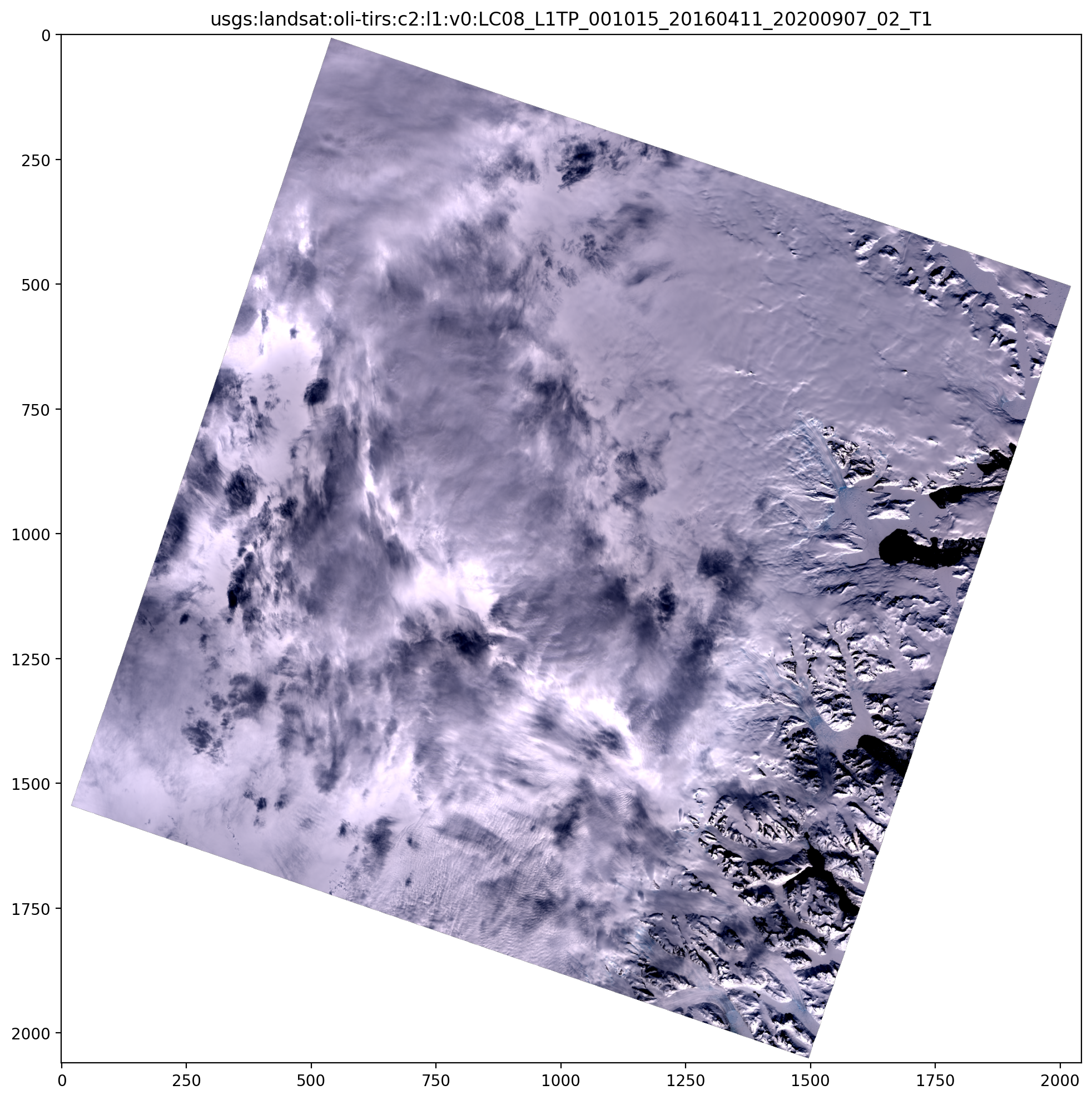
https://descarteslabs-cdn.s3.us-west-2.amazonaws.com/docs/3.0.5/public/_images/catalog_figure24_1.png

The ordering of the axes within the ndarray are (band, y, x) or (band, row, column).

Note that the default geocontext for an image does not specify a resolution, but rather a shape that exactly matches the underlying image data, along with the bounds and crs of the original image. So retrieving with the default context will result in an ndarray that exactly matches the original data, with no warping.

With download() the resulting data is stored in the local filesystem and the name of the file is returned.

>>> import os.path
>>> from descarteslabs.catalog import Image
>>> image = Image.get("usgs:landsat:oli-tirs:c2:l1:v0:LC08_L1TP_001015_20160411_20200907_02_T1")
>>> file = image.download("red green blue", resolution=120)
>>> os.path.exists(file)
True

Rastering image collections

ImageCollection supports several methods for rastering. A variety of parameters used to control the rastering are described in the documentation for ech of these methods.

stack() can be used to raster each of the images in the collection and then stack the resulting 3D arrays into a single 4-dimensional array, with the different images along the first axis in the order they appear in the ImageCollection (i.e. the axes are (image, band, y, x)). Note that rastering the images is performed in parallel, so this is significantly faster than rastering each image in the collection in a loop.

>>> search = Product.get("usgs:landsat:oli-tirs:c2:l1:v0").images()
>>> search = search.intersects(geometry).filter("2017-01-01" <= p.acquired < "2018-01-01")
>>> search = search.filter(p.cloud_fraction <= 0.2)
>>> search = search.sort("acquired")
>>> images = search.collect()
>>> data = images.stack("red green blue", resolution=120)
>>> data.shape
(31, 3, 112, 142)

>>> # display the first few
>>> display(*data[0:4], title=list(images[0:4].each.name), ncols=2)

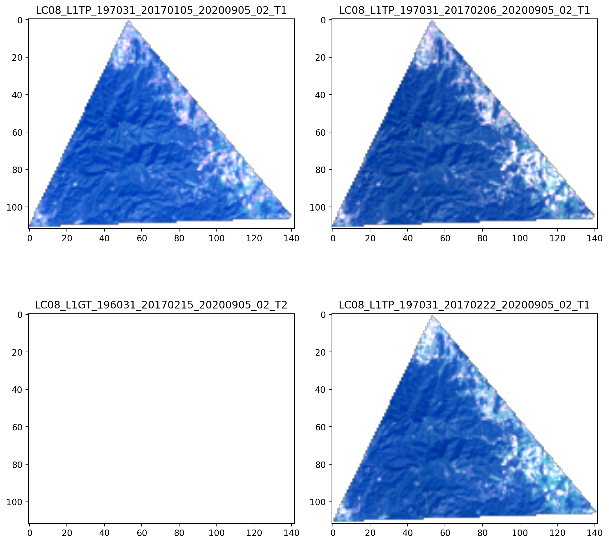
https://descarteslabs-cdn.s3.us-west-2.amazonaws.com/docs/3.0.5/public/_images/catalog_figure26_1.png

Please note the lower-left image, which appears to be blank. This image was selected by the search because the bounding box for the image contains the target geometry. However, the image does not contain valid pixels at that particular location. The mosaic() discussed next will account for this, skipping this particular image and selecting the pixels from another image.

mosaic() can be used to composite the images to form a single image, resulting in a 3D array. A mosaic composite uses, for each pixel location, the pixel value from the last image in the collection containing a valid (unmasked) pixel value at that location. Since individual images may not cover the same pixels this operation is typically used to combine overlapping images to obtain a single complete image. If the image collection is sorted by increasing acquisition date, this means the most recent image wins. You can use the sort() method on the search object to alter the ordering of the images in the collection, or the ~descarteslabs.common.collection.Collection.sort method on the ImageCollection itself to alter the ordering of the images and hence the results of the mosaic operation.

>>> data = images.mosaic("red green blue", resolution=120)
>>> data.shape
(3, 112, 142)

>>> display(data, title="Mosaic")

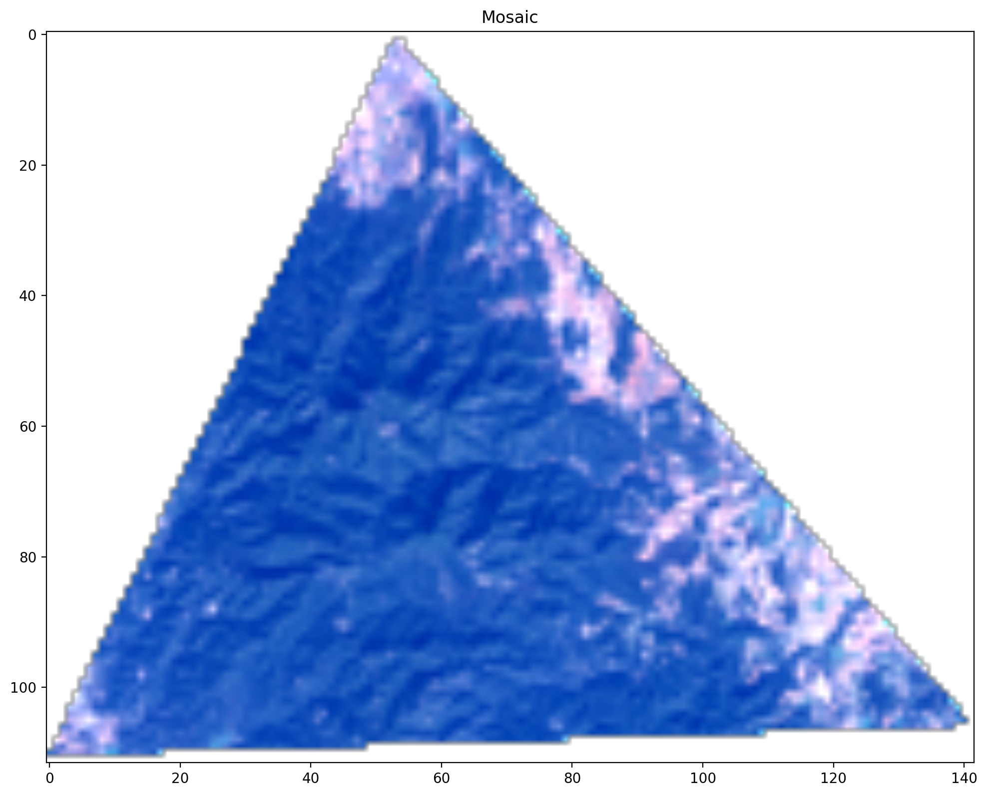
https://descarteslabs-cdn.s3.us-west-2.amazonaws.com/docs/3.0.5/public/_images/catalog_figure27_1.png

See the Compositing Imagery with Catalog example for a more in-depth discussion of compositing by mosaic. Other kinds of compositing are possible but are not directly supported in the rastering engine but are easily achieved using the NumPy package, see the Composite Multi-Product Imagery example for the use of a median composite.

Stacking and compositing can be combined using the stack() method with the flatten parameter. This uses the groupby() method to form a partitioning of the image list into multiple image lists of 1 or more images. Each sub-list is rastered as a composite (mosaic), and the multiple resulting mosaics are stacked. Note in this case that the first dimension of the resulting 4D array is equal to the number of different groups resulting from the flatten operation, and not the number of images in the original ImageCollection.

In this example, we will group the images by the acquisition month. As there is at least one image each month, we end up with twelve partitioned image lists. Thus the resulting stack ends up with twelve mosaics. Note that the flatten operation preserves the original ordering of images within each group, so that if the original image collection is sorted by increasing acquired date, each mosaic will again represent “most recent image wins”.

>>> # Just to see how the images will be grouped
>>> for month, sublist in images.groupby(lambda i: i.acquired.month):
...     print(f"Month {month:02} Images {sublist}")
Month 01 Images ImageCollection of 1 image
  * Dates: Jan 05, 2017 to Jan 05, 2017
  * Products: usgs:landsat:oli-tirs:c2:l1:v0: 1
Month 02 Images ImageCollection of 3 images
  * Dates: Feb 06, 2017 to Feb 22, 2017
  * Products: usgs:landsat:oli-tirs:c2:l1:v0: 3
Month 03 Images ImageCollection of 3 images
  * Dates: Mar 10, 2017 to Mar 26, 2017
  * Products: usgs:landsat:oli-tirs:c2:l1:v0: 3
Month 04 Images ImageCollection of 3 images
  * Dates: Apr 04, 2017 to Apr 20, 2017
  * Products: usgs:landsat:oli-tirs:c2:l1:v0: 3
Month 05 Images ImageCollection of 2 images
  * Dates: May 06, 2017 to May 22, 2017
  * Products: usgs:landsat:oli-tirs:c2:l1:v0: 2
Month 06 Images ImageCollection of 4 images
  * Dates: Jun 07, 2017 to Jun 30, 2017
  * Products: usgs:landsat:oli-tirs:c2:l1:v0: 4
Month 07 Images ImageCollection of 3 images
  * Dates: Jul 09, 2017 to Jul 25, 2017
  * Products: usgs:landsat:oli-tirs:c2:l1:v0: 3
Month 08 Images ImageCollection of 3 images
  * Dates: Aug 10, 2017 to Aug 26, 2017
  * Products: usgs:landsat:oli-tirs:c2:l1:v0: 3
Month 09 Images ImageCollection of 3 images
  * Dates: Sep 02, 2017 to Sep 27, 2017
  * Products: usgs:landsat:oli-tirs:c2:l1:v0: 3
Month 10 Images ImageCollection of 1 image
  * Dates: Oct 29, 2017 to Oct 29, 2017
  * Products: usgs:landsat:oli-tirs:c2:l1:v0: 1
Month 11 Images ImageCollection of 3 images
  * Dates: Nov 14, 2017 to Nov 30, 2017
  * Products: usgs:landsat:oli-tirs:c2:l1:v0: 3
Month 12 Images ImageCollection of 2 images
  * Dates: Dec 16, 2017 to Dec 23, 2017
  * Products: usgs:landsat:oli-tirs:c2:l1:v0: 2

>>> # Do the flatten/mosaic/stack operation
>>> data = images.stack("red green blue", resolution=120, flatten=lambda i: i.acquired.month)
>>> data.shape
(12, 3, 112, 142)

>>> display(*data, title=[f"{m+1:02d}/2017" for m in range(data.shape[0])], ncols=2)

https://descarteslabs-cdn.s3.us-west-2.amazonaws.com/docs/3.0.5/public/_images/catalog_figure28_1.png

ImageCollections support two different forms of download. The download() method works like the stack method, creating one geotiff file for each image in the image collection (but all using the same geocontext), while the download_mosaic() method composites the images in the ImageCollection just like the mosaic() method but results in a single geotiff file rather than an ndarray. The names of the resulting files are generated by default but can also be set explicitly. See the API documentation for further information.

Common Rastering parameters

Many of the rastering methods accept a common set of parameters including geocontext, resolution, processing_level, scaling, data_type and progress. These parameters are treated consistently across the different methods, and merit some explanation and examples.

`geocontext`, `resolution`, `crs`, and `all_touched`

Image and ImageCollection objects have a default geocontext associated with them. The Image.geocontext attribute represents the geometry of the image, while the ImageCollection.geocontext attribute represents the geocontext used in the search that generated the collection, if any. If the geocontext parameter to a rastering method is not specified, this corresponding geocontext of the image or collection will be used by default. The resolution, crs and all_touched parameters can be used to override the corresponding parameters of the geocontext (whether defaulted or explicitly provided).

`processing_level`

The processing_level parameter allows the selection of different processing levels (e.g. toa_reflectance or surface_reflectance) supported by a product and its bands. When specifying a non-default processing level, the resulting data will often have a different data type and scaling than the raw image data. You must consult the processing_levels attribute to determine what processing levels a band supports.

`scaling` and `data_type`

When band raster data is retrieved, it can be scaled and converted to a variety of data types as required by the user. When neither of these parameters are provided, the original band data (or the selected processing_level) is copied into the result without change, while the resulting data type is automatically selected based on the data types of the bands in order to hold all the data without loss of precision or range.

However, the user may specify several different alternative treatments of the band data. One of four automated scaling modes can be specified which direct the operation to rescale the pixel values in each band according to either the range of data in the image or ranges defined in the band attributes and targeting an appropriate output data type.

The raw mode is equivalent to no scaling: the data is preserved as is (after applying any processing_level), and the output data type is selected to hold all the band data without loss of precision or range.

>>> import numpy as np
>>>
>>> product = Product.get("usgs:landsat:oli-tirs:c2:l1:v0")
>>>
>>> bands = {band.name: band for band in product.bands()}
>>> [bands[b].data_type for b in ["red","green","blue"]]
['UInt16', 'UInt16', 'UInt16']

>>> image = list(product.images().filter("2018-07-01" < p.acquired < "2018-09-01").sort("acquired").limit(1))[0]
>>>
>>> arr = image.ndarray(
...     bands="red green blue",
...     resolution=120,
...     scaling="raw"
... )
>>>
>>> arr.dtype
dtype('float64')

>>> np.min(arr)
0.007080000000000003

>>> np.max(arr)
0.23098000000000005

The auto mode automatically scales from the actual range of the band data to the standard display range of ``[0, 255 ``. This scaling is done independently for each band, thus this has the effect of “stretching” the dynamic range of the data in each band.

Note

auto mode cannot be used with any image products supporting processing levels.

>>> dem = Image.get("nasa:aster:gdem3:v1:ASTGTMV003_N64E021_dem.tif")
>>> arr = dem.ndarray(
...     bands="height",
...     scaling="auto"
... )
>>>
>>> arr.dtype
dtype('uint8')

>>> np.min(arr)
0

>>> np.max(arr)
255

The display mode scales from the display_range attribute values on the bands to the standard display range of [0, 255]. Typically this leads to clipping or compression of large pixel values having the effect of brightening the image.

>>> arr = image.ndarray(
...     bands="red green blue",
...     resolution=120,
...     scaling="display"
... )
>>>
>>> arr.dtype
dtype('uint8')

>>> np.min(arr)
5

>>> np.max(arr)
147

The physical mode scales from the data_range attribute values on the bands to the physical_range attribute values on the bands, returning the result as floating point data.

>>> arr = image.ndarray(
...     bands="red green blue",
...     resolution=120,
...     scaling="physical"
... )
>>>
>>> arr.dtype
dtype('float64')

>>> np.min(arr)
0.007080000000000003

>>> np.max(arr)
0.23098000000000005

The scaling parameter can also accept a list of scaling parameters, one for each band in the bands argument. Any of the elements may also be one of the automated mode keywords above, although in general one cannot mix different modes, with the exception of auto and display which can be intermixed. Additionally, when using the tuple notation it is possible to specify a percentage (as a string ending with a ‘%’), and the numeric bound will be computed automatically from the appropriate range from the band’s attributes (e.g. data_range or physical_range). For example, a tuple of ("25%","75%") with a display_range of [0, 4000] will yield (1000, 3000).

>>> # Scale explicitly for normal display range
>>> arr = image.ndarray(
...     bands="red green blue",
...     resolution=120,
...     scaling=[(0, 0.4), (0, 0.4), (0, 0.4)]
... )
>>>
>>> # Scale explicitly for middle half of normal display range
>>> arr = image.ndarray(
...     bands="red green blue",
...     resolution=120,
...     scaling=[("25%", "75%"), ("25%", "75%"), ("25%", "75%")]
... )

Finally, it is possible to pass a dictionary (or other Mapping type) for the scaling parameter. In this case, each band in the list of bands will be looked up in the mapping to find its corresponding scaling value. If the band does not appear in the mapping, and the type of the band is not “mask” or “class”, (band types which are rarely scaled), it will look for the key "default_" in the mapping and use any value it finds. If no value is found, then the scale parameter for the band will be set to None. The use of the mapping type is supported as a convenience; it is possible to define a set of standard scaling parameters by band name once, and then reuse this mapping across many calls to any of the Image or ImageCollection methods which accept the scaling parameter with varying lists of band names.

>>> scaling = {
...     "nir": (0, 10000),
...     "default_": "display"
... }
>>>
>>> rgbn = image.ndarray(
...     bands="red green blue nir",
...     resolution=120,
...     scaling=scaling
... )

There is a convenience method scaling_parameters() which will return the full scales and data_type values which the Image class methods will generate. This can be useful for understanding in detail how scaling is being performed.

>>> image.scaling_parameters(
...     bands="red green blue",
...     scaling="display"
... )
([(0.0, 0.4, 0, 255), (0.0, 0.4, 0, 255), (0.0, 0.4, 0, 255)], 'Byte')

For a full description of the scaling and data_type parameters, please see the documentation of scaling_parameters().

`progress`

The progress parameter can be used to control the display of a progress bar during long-running operations such as ndarray and mosaic. By default it is None, which leaves the progress bar implementation to determine whether or not to display the progress bar based on the environment in which it is running (e.g. is there a terminal?). It can be explicitly set to True or False to override this default determination. Note that when working with a ImageCollection some operations are implemented in a parallel fashion, and in such cases having many progress bars displayed at once may lead to visual clutter, so consider using progress=False if this is a problem.

Creating, uploading and downloading blobs

The mechanics of uploading and downloading blobs is similar to that for images. In order to upload a blob, you must first create a Blob instance, giving it a namespace and name. The namespace will be rewritten, if necessary, to be prefixed with your organization name. The combination of namespace and name must be unique; the name value only needs to be unique with the namespace. Any additional attributes may be assigned at this time. Then, the upload() or upload_data() method is invoked to upload the blob’s data to the Catalog and create the blob entry in the catalog.

To upload from a file (or any file-like Python object such as an io.IOBase):

from descarteslabs.catalog import Blob

>>> blob = Blob(namespace="myproject", name="some/name", geometry=aoi, tags=["important-data"])
>>> blob.upload("path/to/local/file")
Blob: some/name
  id: data/myorg:myproject/some/name
  created: Thu May  4 15:54:52 2023

Alternatively, data can be uploaded from a Python str or bytes object directly:

>>> blob = Blob(name="secrets")
>>> blob.upload_data(json.dumps({"key": "some-key", "secret": "some-secret"}))
Blob: secrets
  id: data/myorg:myuserhash/secrets
  created: Thu May  4 15:55:52 2023

If you know the size (in bytes) or the MD5 checksum hash of the file or data, you can provide these values to the Blob constructor. Once the file or data has been uploaded, the Catalog service will verify that these values match what has been uploaded, and the upload will fail if they do not match. This verification of the correctness of the upload can be especially useful for very large files, which are more prone to corruption due to network problems.

>>> some_data = { "some_key": "some_value" }
>>> data = json.dumps(some_data).encode()
>>> size_bytes = len(data)
>>> hash = hashlib.md5(data).hexdigest()
>>> blob = Blob(namespace="myproject", name="mydata", size_bytes=size_bytes, hash=hash)
>>> blob.upload_data(data)
Blob: mydata
  id: data/myorg:myproject/mydata
  created: Thu May  4 16:01:52 2023

Once a blob has been uploaded, it can be retrieved, searched for, downloaded, or deleted. There are two forms of downloading, one which writes the downloaded data to a local file (or file-like object), and the other which returns the data directly. In the later case, it is also possible to iterate over chunks of bytes, or lines of text, making it possible to stream very large data objects and process bit by bit.

>>> blob = Blob.get("data/myorg:myproject/some/name")

# download to a file
>>> blob.download("path/to/another/file")
'path/to/another/file'

# download to a bytes object
>>> data = blob.data()

# download chunk by chunk
>>> for chunk in blob.iter_data():
...     do_something(chunk)

# download line by line
>>> for line in blob.iter_lines(decode_unicode=True):
...     do_something(line)

Access control

By default only the creator of a product or blob and the administrator for the purchase under which the creator is operating can read and modify it as well as read and modify the bands and images associated with a product. To share access to an with others you can modify its access control lists (ACLs):

>>> product = Product.get("descarteslabs:some-product")
>>> product.readers = ["org:descarteslabs"]
>>> product.writers = ["email:jane.doe@descarteslabs.com", "email:john.daly@gmail.com"]
>>> product.save()

This gives read access to the whole “descarteslabs” organization. All users in that organization can now find the product. This also gives write access to two specific users identified by email. These two users can now update the product and add new images to it. For further information on access control please see the Sharing Resources uide.

Transfering ownership of a blob or product to a new user requires cooperation from both the previous owner and the new owner and is a two-step effort. The first step is for the previous owner to add the new owner to the product:

>>> product.owners.append("user:...")
>>> product.save()

Just a reminder that you cannot use the email: variant as an owner. You will have to request the user id from the new owner and use that instead. (You can find your user id in the profile drop-down on iam.descarteslabs.com).

The second step is for the new owner to remove the previous owner:

>>> product.owners.remove("user:...")
>>> product.save()

Managing products

Creating and updating a product

Before uploading images to the catalog, you need to create a product and declare its bands. The only required attributes for a product are a unique id and a name:

>>> from descarteslabs.catalog import Product
>>> product = Product()
>>> product.id = "guide-example-product"
>>> product.name = "Example product"
>>> product.save()
>>> product.id
'descarteslabs:guide-example-product'
>>> product.created
datetime.datetime(2019, 8, 19, 18, 53, 26, 250005, tzinfo=<UTC>)

save() saves the product to the catalog in the cloud. Note that you get to choose an id for your product but it must be unique within your organization (you get an exception if it’s not). This code example is assuming the user is in the “descarteslabs” organization. The id is prefixed with the organization id on save to enforce global uniqueness and uniqueness within an organization. If you are not part of an organization the prefix will be your unique user id. You can find this unique user id on your IAM page if you click on your name in the upper right.

Every object has a read-only created attribute with the timestamp from when it was first saved.

There are a few more attributes that you can set (see the Product API reference). You can update the product to define the timespan that it covers. This is as simple as assigning attributes and then saving again:

>>> product.start_datetime = "2012-01-01"
>>> product.end_datetime = "2015-01-01"
>>> product.save()
>>> product.start_datetime
datetime.datetime(2012, 1, 1, 0, 0, tzinfo=<UTC>)
>>> product.modified
datetime.datetime(2019, 8, 19, 18, 53, 27, 114274, tzinfo=<UTC>)

A read-only modified attribute exists on all objects and is updated on every save.

Note that all timestamp attributes are represented as datetime instances in UTC. You may assign strings to timestamp attributes if they can be reasonably parsed as timestamps. Once the object is saved the attributes will appear as parsed datetime instances. If a timestamp has no explicit timezone, it’s assumed to be in UTC.

Get existing product or create new one

If you rerun the same code many times and you only want to create the product once, you can use the Product.get_or_create() method. This method will do a lookup, and if not found, will create a new product instance (you can do the same for bands or images):

>>> product = Product.get_or_create("guide-example-product")
>>> product.name = "Example product"
>>> product.save()

This is the equivalent to:

>>> product = Product.get("guide-example-product")
>>> if product is None:
...     product = Product(id="guide-example-product")
>>>  product.name = "Example product"
>>>  product.save()

If the product doesn’t exist yet, it will be created, the name will be assigned, and it will be created by the save. If the product already exists, it will be retrieved. If the assigned name differs, the product will be updated by the save. If everything is identical, the save becomes a noop.

If you like, you can add additional attributes as parameters

>>> product = Product.get_or_create("guide-example-product", name="Example product")
>>> product.save()

Creating bands

Before adding any images to a product you must create bands that declare the structure of the data shared among all images in a product.

>>> from descarteslabs.catalog import SpectralBand, DataType, Resolution, ResolutionUnit
>>> band = SpectralBand(name="blue", product=product)
>>> band.data_type = DataType.UINT16
>>> band.data_range = (0, 10000)
>>> band.display_range = (0, 4000)
>>> band.resolution = Resolution(unit=ResolutionUnit.METERS, value=60)
>>> band.band_index = 0
>>> band.save()
>>> band.id
'descarteslabs:guide-example-product:blue'

A band is uniquely identified by its name and product. The full id of the band is composed of the product id and the name.

The band defines where its data is found in the files attached to images in the product: In this example, band_index = 0 indicates that blue is the first band in the image file, and that first band is expected to be represented by unsigned 16-bit integers (DataType.UINT16).

This band is specifically a SpectralBand, with pixel values representing measurements somewhere in the visible/NIR/SWIR electro-optical wavelength spectrum, so you can also set additional attributes to locate it on the spectrum:

>>> # These values are in nanometers (nm)
>>> band.wavelength_nm_min = 452
>>> band.wavelength_nm_max = 512
>>> band.save()

Bands are created and updated in the same way was as products and all other Catalog objects.

Band types

It’s common for many products to have an alpha band, which masks pixels in the image that don’t have valid data:

>>> from descarteslabs.catalog import MaskBand
>>> alpha = MaskBand(name="alpha", product=product)
>>> alpha.is_alpha = True
>>> alpha.data_type = DataType.UINT16
>>> alpha.resolution = band.resolution
>>> alpha.band_index = 1
>>> alpha.save()

Here the “alpha” band is created as a MaskBand which is by definition a binary band with a data range from 0 to 1, so there is no need to set the data_range and MaskBand display_range attribute.

Setting is_alpha to True enables special behavior for this band during rastering. If this band appears as the last band in a raster operation (such as ImageCollection.mosaic() or ImageCollection.stack()) pixels with a value of 0 in this band will be treated as transparent.

There are five band types which may have some attributes specific to them. The type of a band does not necessarily affect how it is rastered (with the exception of MaskBand.is_alpha described above), it mainly conveys useful information about the data it contains.

All bands have the following attributes in common: id, name, product_id, description, type, sort_order, vendor_order, data_type, nodata, data_range, display_range, resolution, band_index, file_index, jpx_layer_index, vendor_band_name.

SpectralBand: A band that lies somewhere on the visible/NIR/SWIR electro-optical wavelength spectrum. Specificattributes: physical_range, physical_range_unit, wavelength_nm_center, wavelength_nm_min, wavelength_nm_max, wavelength_nm_fwhm, processing_levels, derived_params
MicrowaveBand: A band that lies in the microwave spectrum, often from SAR or passive radar sensors. Specific attributes: frequency, bandwidth, physical_range, physical_range_unit, processing_levels, derived_params
MaskBand: A binary band where by convention a 0 means masked and 1 means non-masked. The data_range and display_range for masks is implicitly [0, 1]. Specific attributes: is_alpha
ClassBand: A band that maps a finite set of values that may not be continuous to classification categories (e.g. a land use classification). A visualization with straight pixel values is typically not useful, so commonly a colormap is used. Specific attributes: colormap, colormap_name, class_labels
GenericBand: A generic type for bands that are not represented by the other band types, e.g., mapping physical values like temperature or angles. Specific attributes: colormap, colormap_name, physical_range, physical_range_unit, processing_levels, derived_params

Note that when retrieving bands using a band-specific class, for example SpectralBand.get(), SpectralBand.get_many() or SpectralBand.search(), you will only retrieve that type of band; any other types will be silently dropped. Using Band.get(), Band.get_many() or Band.search() will return all of the types.

Catalog Product Lifecycle

Products and their associated bands and images only remain accessible while the purchase under which they were created remains active. Once a purchase is completed or expired, the objects can no longer be accessed by the owner or anyone with whom they have been shared. After a period of 90 days, all data will be deleted unless the products have been administratively reassigned to another purchase.

Derived bands

Note

These old-style derived bands are deprecated and support will be removed in the future. They cannot be created by the user.

Deleting bands and products

Any catalog objects (Products, Bands, and Images) can be deleted using the delete method. For example, delete the previously created alpha band:

>>> alpha.delete()
True

A product can only be deleted if it doesn’t have any associated bands or images. Because the product we created still has one band this fails:

>>> product.delete()
Traceback (most recent call last):
  ...
ConflictError: {"errors":[{"detail":"One or more related objects exist","status":"409","title":"Related objects exist"}],"jsonapi":{"version":"1.0"}}

There is a convenience method to delete all bands and images in a product. Be careful as this may delete a lot of data and can’t be undone!

>>> status = product.delete_related_objects()

This kicks off a job that deletes bands and images in the background. You can wait for this to complete and then delete the product:

>>> if status:
...     status.wait_for_completion()
...     if status.status != TaskState.SUCCEEDED:
...         raise RuntimeException("...")
>>> product.delete()

Finding Products by id

You may have noticed that when creating products, the id you provide isn’t the id that is assigned to the object.

>>> product = Product(id="guide-example-product")
>>> product.name = "Example product"
>>> product.save()
>>> product.id
"descarteslabs:guide-example-product"

The id has a prefix added to ensure uniqueness without requiring you to come up with a globally unique name. The ownside of this is you need to remember that prefix when looking up your products later:

# this will return False because the id has a prefix!
>>> Product.exists("guide-example-product")
False

You can use namespace_id() to generate a fully-namespaced product.

>>> product_id = Product.namespace_id("guide-example-product")
>>> product_id
"descarteslabs:guide-example_product"
# this will return True because we now know the prefix!
>>> Product.exists(product_id)
True

Managing images

Apart from searching and discovering data available to you, catalog enables you to upload new images of your own.

Creating images

There are two general mechanisms of creating images in the catalog. Upload is the primary mechanism for creating images, either by uploading supported image files types such as GeoTIFF or JPEG, or by uploading image data in the form of a numpy ndarray. The other mechanism is to create “remote” image entries in the catalog without supplying the actual image data.

Uploading image files

If your data already exists on disk as an image file, usually a GeoTIFF or JPEG file, you can upload it directly.

In the following examples we will upload data with a single band representing the blue light spectrum. First let’s create a product and band corresponding to that:

>>> # Create a product
>>> from descarteslabs.catalog import Band, DataType, Product, Resolution, ResolutionUnit, SpectralBand
>>> product = Product(id="guide-example-product", name="Example product")
>>> product.save()
>>>
>>> # Create a band
>>> band = SpectralBand(name="blue", product=product)
>>> band.data_type = DataType.UINT16
>>> band.data_range = (0, 10000)
>>> band.display_range = (0, 4000)
>>> band.resolution = Resolution(unit=ResolutionUnit.METERS, value=60)
>>> band.band_index = 0
>>> band.save()

Now you create a new image and use image.upload() to upload imagery to the new product. This returns a ImageUpload. Images are uploaded and processed asynchronously, so they are not available in the catalog immediately. With upload.wait_for_completion() we wait until the upload is completely finished.

>>> # Set any attributes that should be set on the uploaded images
>>> image = Image(product=product, name="image1")
>>> image.acquired = "2012-01-02"
>>> image.cloud_fraction = 0.1
>>>
>>> # Do the upload
>>> image_path = "docs/guides/blue.tif"
>>> upload = image.upload(image_path)
>>> upload.wait_for_completion()
>>> upload.status
'success'

Attributes that can be derived from the image file, such as the georeferencing, will be assigned to the image during the upload process. But you can set any additional Image attributes such as acquired and cloud_fraction when you create the image (as was done with image.cloud_fraction above).

Note that this code makes a number of assumptions:

A GeoTIFF exists locally on disk at the path docs/guides/blue.tiff from the current directory.
The GeoTIFF’s only band matches the blue band we created (for example, it has an unsigned 16-bit integer data type).
The GeoTIFF is correctly georeferenced.

Uploading ndarrays

Often, when creating derived product - for example, running a classification model on existing data - you’ll have a NumPy array (often referred to as “ndarrays”) in memory instead of a file written to disk. In that case, you can use upload_ndarray(). This method behaves like Image upload(), with one key difference: you must provide georeferencing attributes for the ndarray.

Georeferencing attributes are used to map between geospatial coordinates (such as latitude and longitude) and their corresponding pixel coordinates in the array. The required attributes are:

An affine geotransform in GDAL format (the geotrans attribute)
A coordinate reference system definition, preferrably as an EPSG code (the cs_code attribute) or alternatively as a string in PROJ.4 or WKT format (the projection attribute)

If the ndarray you’re uploading was rastered through the the platform, this information is easy to get. When rastering you also receive a dictionary of metadata that includes both of these parameters. Using the Image.ndarray(), you have to set raster_info=True; with Raster.ndarray(), it’s always returned.

The following example puts these pieces together. This extracts the blue band from a Landsat 8 scene at a lower resolution and uploads it to our product:

>>> from descarteslabs.catalog import OverviewResampler
>>>
>>> image = descarteslabs.catalog.Image.get("usgs:landsat:oli-tirs:c2:l1:v0:LC08_L1TP_163068_20181025_20200830_02_T1")
>>> ndarray, raster_meta = image.ndarray("blue", resolution=60, raster_info=True)
>>> image2 = Image(product=product, name="image2")
>>> image2.acquired = image.acquired
>>> upload2 = image2.upload_ndarray(
...     ndarray,
...     raster_meta=raster_meta,
...     # create overviews for 120m and 240m resolution
...     overviews=[2, 4],
...     overview_resampler=OverviewResampler.AVERAGE,
... )
...
>>> upload2.wait_for_completion()
>>> upload2.status
'success'

The rastered ndarray here is a three-dimensional array in the shape (band, x, y) - the first axis corresponds to the band number. upload_ndarray() expects an array in that shape and will raise a warning if thinks the shape of the array is wrong. If the given array is two-dimensional it will assume you’re uploading a single band image.

This also specifies typically useful values for overviews and overview_resampler. Overviews allow the platform to raster your image faster at non-native resolutions, at the cost of more storage and a longer initial upload processing time to calculate the overviews.

The overviews argument specifies a list of up to 16 different resolution magnification factors to calulate overviews for. E.g. overviews=[2,4] calculates two overviews at 2x and 4x the native resolution. The overview_resampler argument specifies the algorithm to use when calculating overviews, see Image upload_ndarray() for which algorithms can be used.

Updating images

The image created in the previous example is now available in the Catalog. We can look it up and update any of its attributes like any other catalog object:

>>> image2 = Image.get(image2.id)
>>> image2.cloud_fraction = 0.2
>>> image2.save()

To update the underlying file data, you will need to upload a new file or ndarray. However you must utilize a new unsaved Image instance (using the original product id and image name) along with the overwrite=True parameter. The reason for this is the original image which is now saved in the catalog contains many computed values, which may be different from those which would be computed from the new upload. There is no way for the catalog to know if you intend to reuse the original values or compute new values for these attributes. Also be aware that using the overwrite=True parameter can lead to data cache inconsistencies in the platform which may last a while, so it should be used sparingly with no expectation of seeing the updated data immediately.

Uploading many images

If you are going to be uploading a large number of images - especially if you are doing so from inside a set of tasks running in parallel, it is better to avoid calling the wait_for_completion() method immediately after initiating each upload. You can instead use the ability to query uploads to determine later on what has succeeded, failed, or is still running at a later time. This has advantages both in within a loop, where you don’t have to waste time waiting for each one, and in the tasks framework, where waiting inside of many tasks wastes resources and slows down the entire job.

As an example, if you have used either a loop or a task group to upload a bunch of images to a single product, you can use a pattern like the following to gather up the results.

>>> for upload in product.image_uploads().filter():
...     if upload.status not in (
...         ImageUploadStatus.SUCCESS,
...         ImageUploadStatus.FAILURE,
...         ImageUploadStatus.CANCELED
...     ):
...         upload.wait_for_completion()
...     # do whatever you want here ...

Note that the above will return all uploads that you initiated on the product that are still being tracked; you may wish to do additional filtering on the created timestamp or other attribute to narrow the search.

Troubleshooting uploads

The ImageUpload returned from upload() and upload_ndarray() provides status information on the image upload.

In the following example we upload an invalid file (it’s empty), so we expect the upload to fail. Additional information about the failure should be available in the events attribute, which will contain a list of error records:

>>> import tempfile
>>> invalid_image_path = tempfile.mkstemp()[1]
>>> with open(invalid_image_path, "w"): pass
>>>
>>> image3 = Image(product=product, name="image3", acquired="2012-03-01")
>>> upload3 = image3.upload(invalid_image_path)
>>> upload3.status
'pending'
>>>
>>> upload3.wait_for_completion()
>>> upload3.status
'failure'
>>> upload3.events
[ImageUploadEvent:
  component: yaas
  component_id: yaas-release-cc95fb75-gwxvr
  event_datetime: 2020-01-09 14:12:35.2387465+00:00
  event_type: queue
  id: 13
  message: message-id=XXXXXXX
  severity: INFO
ImageUploadEvent:
  component: yaas_worker
  component_id: metadata-ingest-v2-release-57fbf59cc-rvxwg
  event_datetime: 2020-01-09 14:12:35.756811+00:00
  event_type: run
  id: 14
  message: Running
  severity: INFO
ImageUploadEvent:
  component: IngestV2Worker
  component_id: metadata-ingest-v2-release-57fbf59cc-rvxwg
  event_datetime: 2020-01-09 14:12:35.756811+00:00
  event_type: complete
  id: 15
  message: InvalidFileError: Cannot determine file information, missing the following properties for <...>: ['size']
  severity: ERROR
]

Uploads also contain a list of events pertaining to the upload. These can be useful for understanding or diagnosing problems.

You can also list any past upload results with Product.image_uploads() and Image.image_uploads(). Note that upload results are currently not stored indefinitely, so you may not have access to the full history of uploads for a product or image.

>>> for upload in product.image_uploads():
...     print(upload.id, upload.image_id, upload.status)
...
10635 descarteslabs:guide-example-product:image1 success
10702 descarteslabs:guide-example-product:image2 success
10767 descarteslabs:guide-example-product:image3 failure

Alternatively you can filter the list by attributes such as the status.

>>> for upload in product.image_uploads().filter(properties.status == ImageUploadStatus.FAILURE):
...     print(upload.id, upload.image_id, upload.status)
...
10767 descarteslabs:guide-example-product:image3 failure

In the event that you experience an upload failure, and the error(s) don’t make it clear what you need to do to fix it you should include the upload object id and any events and errors associated with it when you communicate with the Descartes Labs support team.

Tags & extra attributes

The image attributes you can set, filter by and sort on are documented on the Image class. If you have other structured metadata to attach with your images you can use extra_properties:

>>> image2.extra_properties = {
...     "processing_time": 120,
...     "quality": 0.5,
...     "reviewer": "joe@acme.com",
... }
...
>>> image2.save()

extra_properties is a dictionary with string keys and values of any type that can be JSON-serialized (booleans, numbers, strings, lists, dictionaries).

Note that you cannot filter or sort images by extra_properties. Use tags if you have a finite discrete number of custom values you’d like to filter by:

>>> image2.tags = ["temporary", "guide"]
>>> image2.save()
>>>
>>> # Find all images in the product tagged "temporary"
>>> search = product.images().filter(p.tags == "temporary")
>>> for image in search:
...     print(image)
Image:
  id: descarteslabs:guide-example-product:image2
  product: descarteslabs:guide-example-product
  created: Mon Aug 19 18:53:43 2019

Remote images

In addition to hosting rasterable images with file data attached, the catalog also supports images where the underlying raster data is not directly available. These remote images cannot be rastered but can be searched for using the catalog. This is useful for a couple of scenarios:

A product of images that have not been consistently processed, optimized or georegistered in a way that prevents them from being rastered by the platform, for example raw imagery taken in unprocessed form from a sensor. Such a product can serve as the basis for higher-level products that have been processed consistently from the raw imagery.
A product of images for which file data exist somewhere outside the platform but has not been uploaded or only partly uploaded into the platform. This gives users the chance to browse the full metadata of images and then make decisions about what file data should be uploaded on demand.

To create a remote image set storage_state to "remote". The only other required attributes for remote images are acquired and Image geometry to anchor them in time and space. No bands are required for a product holding only remote images.

>>> from descarteslabs.catalog import Product, Image, StorageState
>>> product = Product(id="guide-example-raw", name="Raw product")
>>> product.save()
>>>
>>> geometry = {
...     "type": "Polygon",
...     "coordinates": [[
...         [7.488099932670593, 46.95386728954941],
...         [7.488352060317992, 46.953656742419255],
...         [7.488429844379425, 46.953916722233814],
...         [7.488099932670593, 46.95386728954941]
...     ]]
... }
...
>>> image = Image(product=product, name="raw-image")
>>> image.storage_state = StorageState.REMOTE
>>> image.acquired = "2018-04-12"
>>> image.geometry = geometry
>>> image.save()

If some form of URL referencing the remote image is available, attach it through the Image files attribute using a File:

>>> from descarteslabs.catalog import File
>>> image.files = [File(href="http://remote.server.com/path/image.tiff")]
>>> image.save()

Porting from Scenes to Catalog

As of Python client version 1.12.0, the abilities to raster images and collections of images was migrated from the Scenes API to the Catalog API. As of this release, the Scenes API is now deprecated and will be removed in a future release. This addendum provides some guidance on how to port client code from using the Scenes API to the equivalent capabilities of the Catalog API.

Search

The search APIs of the Scenes client are now superceded by the search APIs of Catalog. In general, the search capabilities in Catalog are more comprehensive and powerful than those in Scenes, allowing finer control over filtering, sorting, and iteration.

As a comprehensive example, the following search using the Scenes API:

>>> from descarteslabs import scenes

>>> scene_collection, ctx = scenes.search(
...     geometry,
...     products="usgs:landsat:oli-tirs:c2:l1:v0",
...     cloud_fraction=0.25,
...     start_datetime="2013-07-01",
...     end_datetime="2013-09-01",
...     sort_field="acquired",
...     sort_order="asc",
...     limit=10
... )

can be reproduced using Catalog as:

>>> from descarteslabs.catalog import *
>>> from descarteslabs.catalog import properties as p

>>> image_collection = (
...     Product.get("usgs:landsat:oli-tirs:c2:l1:v0").images()
...     .intersects(geometry)
...     .filter(p.cloud_fraction < 0.25)
...     .filter("2013-07-01" <= p.acquired < "2013-09-01")
...     .sort("acquired")
...     .limit(10)
... ).collect()

Note that the GeoContext returned by scenes.search() is now available as the default GeoContext on returned ImageCollection. Also note that in Catalog the default sorting is by object id, so you must explicitly sort by the acquired date to replicate the default behavior of the scenes.search() function.

Searching for products and bands is similarly handled by Catalog search:

>>> products = scenes.search_products(text="landsat", limit=10)

>>> for product in products:
...     bands = scenes.search_bands(product.id)

can be written as:

>>> products = Product.search().find_text("landsat").limit(10):

>>> for product in products:
...     bands = product.bands().collect()

with products being a ProductCollection rather than a list of DotDict.

Image vs Scene

The Image class now implements all the rastering methods of the Scene class in a fully compatible way. The one difference is that the Image class supports the default Image geocontext attribute so that it is not required to supply a geocontext to the rastering method, and as a convenience, the resolution parameter may be used to update the desired resolution on the geocontext.

>>> scene, ctx = scenes.Scene.from_id("usgs:landsat:oli-tirs:c2:l1:v0:LC08_L1TP_163068_20181025_20200830_02_T1")
>>> lowres_ctx = ctx.assign(resolution=120)
>>> arr = scene.ndarray("red green blue", lowres_ctx)

becomes:

>>> image = Image.get("usgs:landsat:oli-tirs:c2:l1:v0:LC08_L1TP_163068_20181025_20200830_02_T1")
>>> arr = image.ndarray("red green blue", resolution=120)

ImageCollection vs SceneCollection

Similarly, the descarteslabs.catalog.ImageCollection class now implements all the rastering methods of the SceneCollection class in a fully compatible way. And again, the one difference is that the ImageCollection class supports the default geocontext attribute so that it is not required to supply a geocontext to the rastering method, and as a convenience, the resolution parameter may be used to update the desired resolution on the geocontext. The sole exception is when the ImageCollection was obtained without use of the intersects() method, in which case there will be no default geocontext and the user must supply an appropriate GeoContext via the geocontex parameter.

>>> scene_collection, ctx = scenes.search(
...     geometry,
...     products="usgs:landsat:oli-tirs:c2:l1:v0",
...     start_datetime="2018-06-01",
...     end_datetime="2018-07-01",
... )
>>> lowres_ctx = ctx.assign(resolution=120)
>>> arr = scene_collection.mosaic("red green blue", lowres_ctx)

becomes:

>>> search = Product.get("usgs:landsat:oli-tirs:c2:l1:v0").images()
>>> search = search.intersects(geometry).filter("2018-06-01" <= p.acquired < "2018-07-01")
>>> search = search.sort("acquired")
>>> image_collection = search.collect()
>>> arr = image_collection.mosaic("red green blue", resolution=120)

Porting from Storage to Catalog

For users migrating from the legacy Google Cloud environment to the new AWS environment, the Catalog Blob replaces the legacy ``Storage` API. Whereas the legacy Storage API is nothing more than a simple key-value store, the Catalog Blob offers a fully indexed and searchable (by attributes) catalog of stored data, and thus offers a much richer interface. Porting code from the legacy Storage API to Catalog Blobs should be a simple exercise.

Legacy code to upload a file might look like this:

>>> from descarteslabs import storage
>>> storage.set_file("some-key", "filename")

The corresponding operation using blobs would look like this:

>>> from descarteslabs.catalog import Blob
>>> Blob(name="some-key").upload("filename")
Blob: some-key
  id: data/myorg:myuserhash/some-key
  created: Thu May  4 15:54:52 2023

(Note that the namespace, not specified above, will default to the user’s organization.)

Legacy code to upload a string or bytes might look like this:

>>> from descarteslabs import storage
>>> storage.set("some-key", "some data")

The corresponding operation using blobs would look like this:

>>> from descarteslabs.catalog import Blob
>>> Blob(name="some-key").upload_data("some data")
Blob: some-key
  id: data/myorg:myuserhash/some-key
  created: Thu May  4 15:55:52 2023

To download previously uploaded data to a file, legacy code might look like this:

>>> from descarteslabs import storage
>>> storage.get_file("some-key", "filename")

The corresponding operation using blobs would look like this:

>>> from descarteslabs.catalog import Blob
>>> Blob.get(name="some-key").download("filename")
'filename'

To download previosly uploaded data directly, legacy code might look like this:

>>> from descarteslabs import storage
>>> data = storage.get("some-key")

The corresponding operation using blobs would look like this:

>>> from descarteslabs.catalog import Blob
>>> data = Blob.get("data/myorg:myuserhash/some-key").data().decode()

(As Blob data is inherently bytes, the .decode() will convert the retrieved bytes to a string, as the legacy Storage client always did.)

The legacy Storage API provides list() and iter_list() methods providing the keys of all items, possibly matching a prefix. This capability is replaced with the generalized search capabilities of Blobs.

Catalog

Concepts

Images

ImageCollections

Bands

Products

Blobs

Searching the catalog

Finding products

Filtering, sorting, and limiting

Text search

Lookup by id and object relationships

Finding images

Image filters

ImageCollections

Image summaries

Finding blobs

Lookup by id

Blob filters

Blob summaries

Rastering imagery

Rastering images

Rastering image collections

Common Rastering parameters

geocontext, resolution, crs, and all_touched

processing_level

scaling and data_type

progress

Creating, uploading and downloading blobs

Access control

Managing products

Creating and updating a product

Get existing product or create new one

Creating bands

Band types

Catalog Product Lifecycle

Derived bands

Deleting bands and products

Finding Products by id

Managing images

Creating images

Uploading image files

Uploading ndarrays

Updating images

Uploading many images

Troubleshooting uploads

Tags & extra attributes

Remote images

Porting from Scenes to Catalog

Search

Image vs Scene

ImageCollection vs SceneCollection

Porting from Storage to Catalog

`geocontext`, `resolution`, `crs`, and `all_touched`

`processing_level`

`scaling` and `data_type`

`progress`