GeoContext

GeoContext objects provide for the consistent specification of geospatial properties including coordinates, coordinate systems, and resolution across all parts of the descarteslabs library. The AOI, DLTile and XYZTile classes provide specializations of GeoContext for specific purposes.

While it is possible to construct a GeoContext explicitly, they are often obtained via the geocontext attribute of the raw imagery or from the geocontext attribute resulting from a search for imagery.

This guide will demonstrate some of the basic operations that are possible with GeoContext objects.

Working with default GeoContext objects

When using the Catalog API to retrieve images or image collections, a default context is available as the corresponding geocontext attribute.

For an Image object this attribute is a GeoContext object with bounds representing the footprint of the underlying image data.

When searching for imagery, the intersects() method can be used to specify a geospatial area of interest. This may be done using a GeoContext object, a GeoJSON-compatible Python dictionary, or a Shapely geometry (see https://shapely.readthedocs.io/en/stable/manual.html). GeoJSON and Shapely geometries are always interpreted in a WGS84 (EPSG:4326) coordinate system, while a GeoContext can use any supported coordinate system (expressible as an EPSG code or a Proj4 or WKT string). It is quite typical to use a simple GeoJSON bounding box ("type": "Polygon") as a starting point. The default geocontext attribute of the resulting ImageCollection object will be converted to its corresponding GeoContext representation.

The lone case where a geocontext is not available is as the result of an image search which does not specify any area of interest (as the images could potentially come from any region of the globe).

Here we retrieve a single image to work with in the subsequent examples.

>>> from descarteslabs.geo import GeoContext, AOI, DLTile, XYZTile
>>> from descarteslabs.catalog import Image
>>> from descarteslabs.utils import display
>>> image = Image.get("usgs:landsat:oli-tirs:c2:l1:v0:LC08_L1TP_163068_20181025_20200830_02_T1")
>>> image.geocontext
AOI(geometry=<POLYGON ((41...12.605, 41...>,
    resolution=None,
    crs='EPSG:32638',
    align_pixels=False,
    bounds=(128092.5, -1395922.5, 355522.5, -1164592.5),
    bounds_crs='EPSG:32638',
    shape=(7711, 7581),
    all_touched=False)

By default this GeoContext is used for rastering operations (it is not recommended that you actually attempt this example code; the resulting image is > 1GB in size and will likely timeout and fail):

>>> arr = image.ndarray("red green blue")
>>> arr.shape
(3, 7711, 7581)

GeoContext objects are immutable; instead, you create copies with new values using the assign() method or subtile() method of the DLTile class.

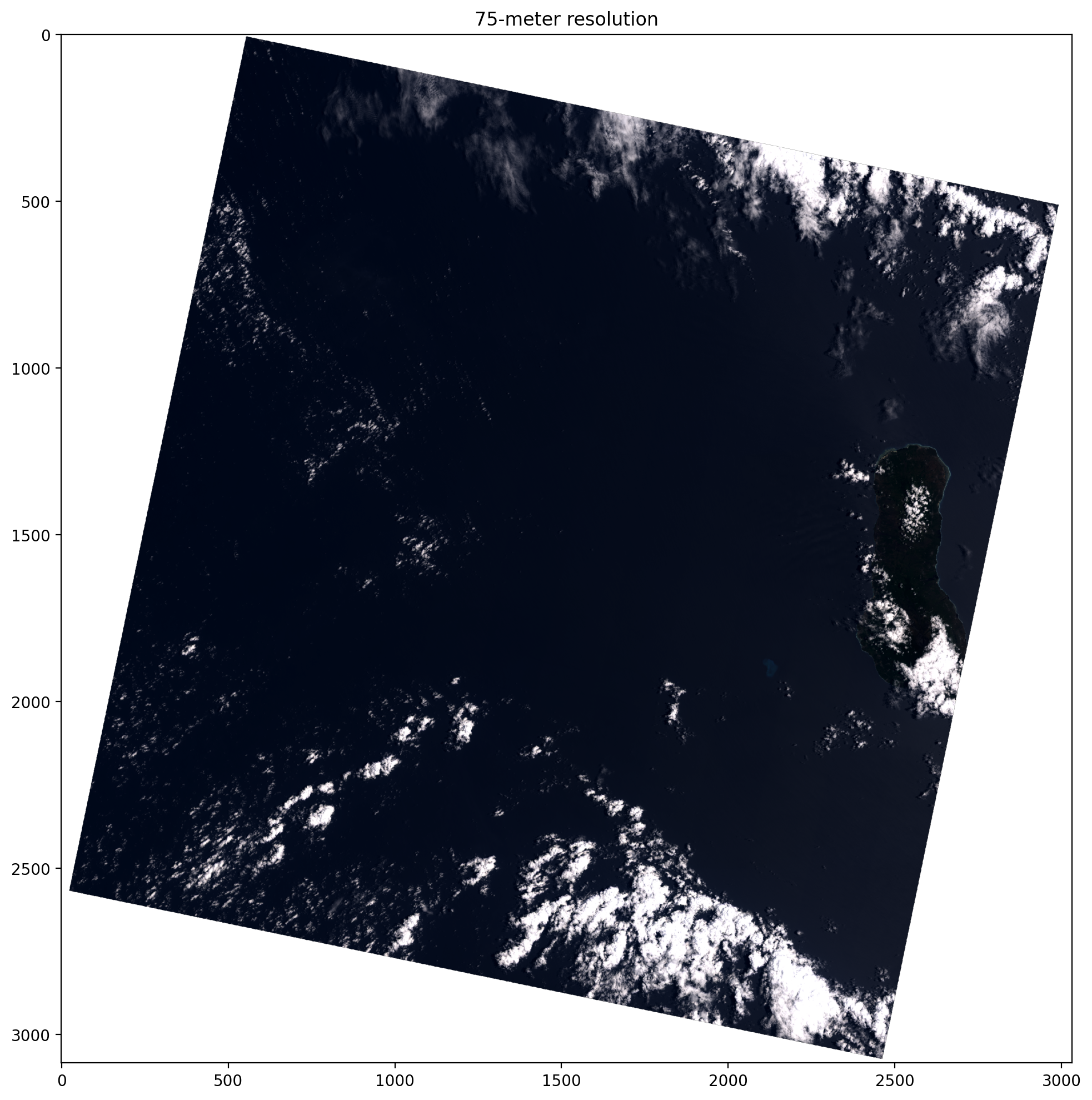
Let’s create a new GeoContext with a lower resolution to load images faster:

>>> lowres = image.geocontext.assign(resolution=75)
>>> lowres_arr = image.ndarray("red green blue", lowres)
>>> display(lowres_arr, title="75-meter resolution")

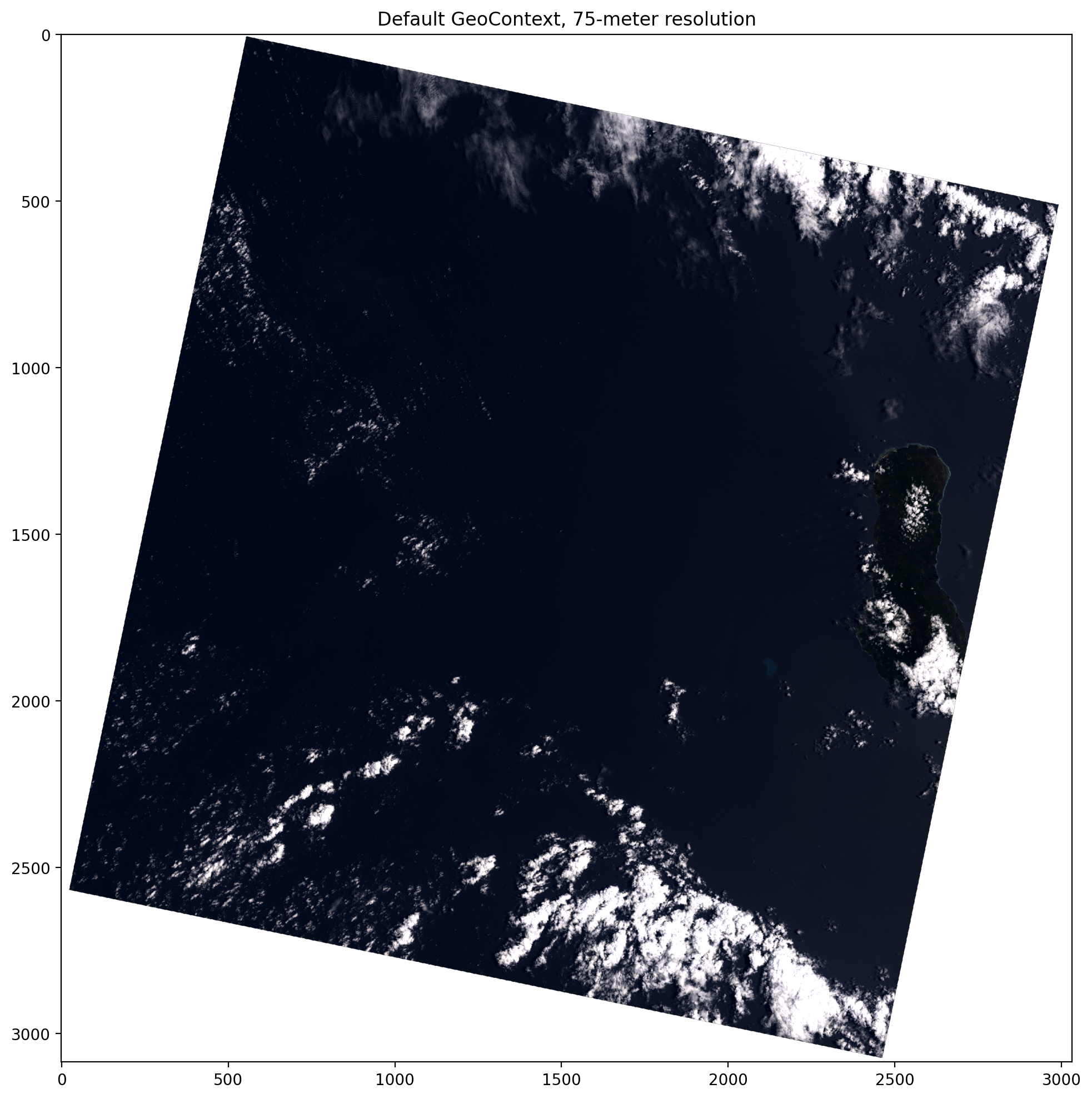
Note that for convenience, the same thing can be achieved by using the default geocontext along with with resolution parameter:

>>> lowres_arr = image.ndarray("red green blue", resolution=75)
>>> display(lowres_arr, title="Default GeoContext, 75-meter resolution")

AOI

The AOI class can be used to define an arbitrary geospatial area of interest. An area of interest consists of a geometry, specified as a GeoJSON Python dictionary or anything implementing the standard __geo_interface__ API which includes Shapely geometries and all GeoContext types, and an associated coordinate reference system (crs) in which to interpret the geometry. For rastering purposes, an AOI must also specify a resolution, and optionally may specify a shape (e.g. X pixels by Y pixels) and a bounds which may itself be expressed in a different coordinate reference system (bounds_crs). Finally, several parameters controlling the rasterizing process are included as properties of the AOI although they have no geospatial meaning. These include align_pixels and all_touched, which are described in the AOI API documentation.

The geometry of an AOI indicates the desired area to be search or rasterized. It may either fully contain, partially intersect, or be fully contained by the area covered by any specific image. Only those portions of an image which are contained within the AOI will be rasterized. The bounds of an AOI represent the the retangular area to be emcompassed by the resulting image after rastering. Portions of the resulting image which lie outside of the geometry but within the bounds will be masked in the resulting image. This will be demonstrated below.

You can create an AOI explicitly. We’ll make a new polygon half the size of the example image’s full extent, and then use a Web Mercator (EPSG:3857) projection (see see http://epsg.io/3857). As you can see in the resulting image, compared to that above, only the center half of the image has been rastered.

>>> import shapely.affinity
>>>
>>> new_cutline = shapely.affinity.scale(image.geometry, xfact=0.5, yfact=0.5)
>>> webmerc_cutline_aoi = AOI(
...     geometry=new_cutline,
...     resolution=75,
...     crs="EPSG:3857"
... )
>>>
>>> webmerc_cutline_arr = image.ndarray("red green blue", webmerc_cutline_aoi)
>>> display(webmerc_cutline_arr, title="Same image, with cutline and Web Mercator")

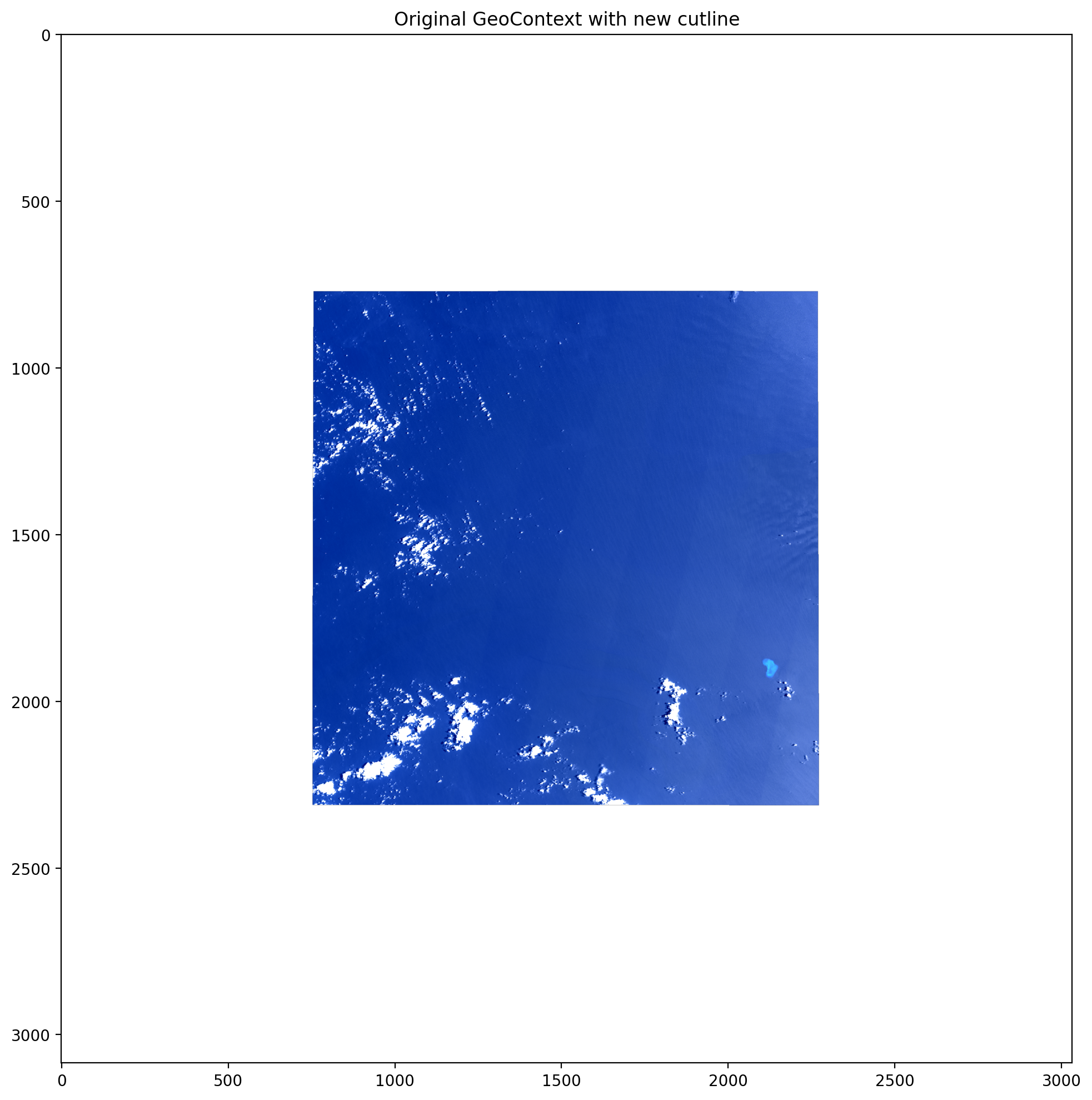
Let’s assign our new cutline to the default GeoContext to see the difference between the coordinate reference systems. Note that by creating a new AOI using assign() we retain the original bounds for the rastered image, resulting in the empty space around around the sides of the image:

>>> with_cutline = lowres.assign(geometry=new_cutline)
>>> with_cutline_arr = image.ndarray("red green blue", with_cutline)
>>> display(with_cutline_arr, title="Original GeoContext with new cutline")

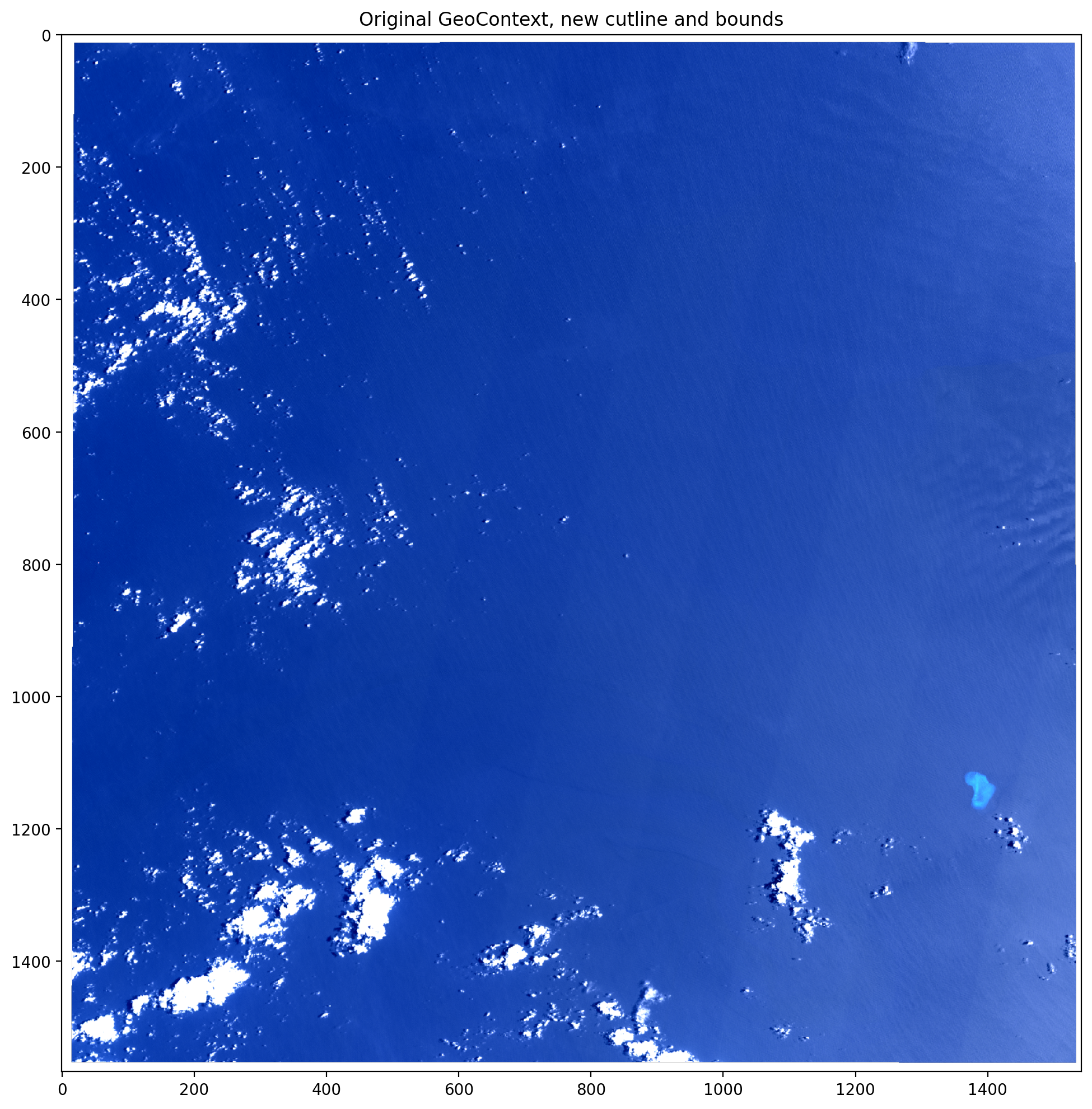
Bounds determine the x-y extent that’s rasterized; geometry just clips within that. You can pass bounds="update" to compute new bounds when assigning a new geometry.

>>> cutline_bounds = lowres.assign(geometry=new_cutline, bounds="update")
>>> cutline_bounds_arr = image.ndarray("red green blue", cutline_bounds)
>>> display(cutline_bounds_arr, title="Original GeoContext, new cutline and bounds")

Bounds can be expressed in any coordinate reference system, set in bounds_crs. They’re typically either in the native CRS of the image, or in WGS84 when clipping to a geometry. Note that when computing bounds from a geometry, bounds_crs is automatically set to EPSG:4326 (short for WGS84 lat-lon coordinates), since that’s the CRS in which the geometry is also defined.

DLTile

The DLTile provides a mechanism for generating square tiles that cover an area of interest using a fixed grid system. DLTiles are based on UTM zones and are especially useful for decomposing a large area of interest into bite-sized chunks that can be rastered and processed in parallel. DLTiles are defined by a small set of parameters which are easily expressed as a key enabling the specification of tiles to be trivially passed around as simple strings.

DLTiles have a tilesize defining the size of the tile in terms of pixels and a corresponding resolution expressed in meters. Every DLTile has a zone, ti, and tj coordinate triple which locates the tile within a grid aligned with the center meridian of the corresponding UTM zone (it should be noted that DLTiles utilize only the 60 North UTM zones, extending their indexing into the southern hemisphere, and are regular in the Nordic region unlike the standard UTM zones). DLTiles also support extra padding around the outside of the square which is useful to support overlapping tiles and algorithmic convolutions which require neighboring pixels.

DLTiles are typically generated to cover a desired AOI, or generated singly to contain a single lat-lon point, or from a supplied DLTile key string. When generating tiles to cover an AOI which spans more than one UTM zone, some of the resulting tiles will necessarily overlap along the zone boundary meridians, due to the nature of UTM coordinate systems.

Create a DLTile from our above geometry:

>>> tiles = DLTile.from_shape(
...     new_cutline,
...     resolution=75,
...     tilesize=256, pad=16
... )
>>>
>>> len(tiles)
49

>>> tile0_arr = image.ndarray("red green blue", tiles[0])
>>> tile0_arr.shape
(3, 288, 288)

>>> tile1_arr = image.ndarray("red green blue", tiles[1])
>>> tile1_arr.shape
(3, 288, 288)

>>> display(tile0_arr, tile1_arr, title=[tiles[0].key, tiles[1].key], ncols=2)

Note that the returned arrays are 288 pixels on a side, due to the 256 pixel tile size plus the 16 pixels of padding all the way around.

The subtile() method can be used to generate new tiles from existing tiles, by subdividing. Here’s an example that creates 4 tiles from a single tile, keeping the tile size but halving the resolution:

>>> tile = tiles[0]
>>> tile
DLTile(key='256:16:75.0:38:-12:-70',
       resolution=75.0,
       tilesize=256,
       pad=16,
       crs='EPSG:32638',
       bounds=(268400.0, -1345200.0, 290000.0, -1323600.0),
       bounds_crs='EPSG:32638',
       geometry=<POLYGON ((42...1.965, 42....>,
       zone=38,
       ti=-12,
       tj=-70,
       geotrans=(268400.0, 75.0, 0.0, -1323600.0, 0.0, -75.0),
       proj4='+proj=utm +z...s=m +no_defs ',
       wkt='PROJCS["WGS ...SG","32638"]]',
       all_touched=False)

>>> for subtile in tile.subtile(2, resolution=tile.resolution/2):
...     print(subtile)
DLTile(key='256:16:37.5:38:-24:-139',
       resolution=37.5,
       tilesize=256,
       pad=16,
       crs='EPSG:32638',
       bounds=(269000.0, -1335000.0, 279800.0, -1324200.0),
       bounds_crs='EPSG:32638',
       geometry=<POLYGON ((42...-11.971, 4...>,
       zone=38,
       ti=-24,
       tj=-139,
       geotrans=(269000.0, 37.5, 0.0, -1324200.0, 0.0, -37.5),
       proj4='+proj=utm +z...s=m +no_defs ',
       wkt='PROJCS["WGS ...SG","32638"]]',
       all_touched=False)
DLTile(key='256:16:37.5:38:-23:-139',
       resolution=37.5,
       tilesize=256,
       pad=16,
       crs='EPSG:32638',
       bounds=(278600.0, -1335000.0, 289400.0, -1324200.0),
       bounds_crs='EPSG:32638',
       geometry=<POLYGON ((42...11.971, 42...>,
       zone=38,
       ti=-23,
       tj=-139,
       geotrans=(278600.0, 37.5, 0.0, -1324200.0, 0.0, -37.5),
       proj4='+proj=utm +z...s=m +no_defs ',
       wkt='PROJCS["WGS ...SG","32638"]]',
       all_touched=False)
DLTile(key='256:16:37.5:38:-24:-140',
       resolution=37.5,
       tilesize=256,
       pad=16,
       crs='EPSG:32638',
       bounds=(269000.0, -1344600.0, 279800.0, -1333800.0),
       bounds_crs='EPSG:32638',
       geometry=<POLYGON ((42...-12.057, 4...>,
       zone=38,
       ti=-24,
       tj=-140,
       geotrans=(269000.0, 37.5, 0.0, -1333800.0, 0.0, -37.5),
       proj4='+proj=utm +z...s=m +no_defs ',
       wkt='PROJCS["WGS ...SG","32638"]]',
       all_touched=False)
DLTile(key='256:16:37.5:38:-23:-140',
       resolution=37.5,
       tilesize=256,
       pad=16,
       crs='EPSG:32638',
       bounds=(278600.0, -1344600.0, 289400.0, -1333800.0),
       bounds_crs='EPSG:32638',
       geometry=<POLYGON ((42...-12.058, 4...>,
       zone=38,
       ti=-23,
       tj=-140,
       geotrans=(278600.0, 37.5, 0.0, -1333800.0, 0.0, -37.5),
       proj4='+proj=utm +z...s=m +no_defs ',
       wkt='PROJCS["WGS ...SG","32638"]]',
       all_touched=False)

And here’s an example that creates a single new tile that covers the same area as the original tile but doubles the resolution:

>>> for subtile in tile.subtile(1, resolution=tile.resolution*2):
...     print(subtile)
DLTile(key='128:16:150.0:38:-12:-70',
       resolution=150.0,
       tilesize=128,
       pad=16,
       crs='EPSG:32638',
       bounds=(267200.0, -1346400.0, 291200.0, -1322400.0),
       bounds_crs='EPSG:32638',
       geometry=<POLYGON ((42...-11.954, 4...>,
       zone=38,
       ti=-12,
       tj=-70,
       geotrans=(267200.0, 150.0, 0.0, -1322400.0, 0.0, -150.0),
       proj4='+proj=utm +z...s=m +no_defs ',
       wkt='PROJCS["WGS ...SG","32638"]]',
       all_touched=False)

XYZTile

The XYZTile provides a mechanism for generating web mercator tiles as those used in web maps. The tiles are always 256x256 pixels, in the spherical Mercator or “Web Mercator” coordinate reference system (EPSG:3857).

Because these tiles are fixed by their XYZ coordinates and the 256x256 tile size, they cannot be altered via the assign method.

>>> tile = XYZTile(14, 27, 5)
>>> print(shapely.geometry.mapping(tile.geometry))
{'type': 'Polygon', 'coordinates': (((-11.25, -79.17133464081945), (-11.25, -76.84081641443098), (-22.5, -76.84081641443098), (-22.5, -79.17133464081945), (-11.25, -79.17133464081945)),)}

>>> print(tile.crs)
EPSG:3857