Dynamic Compute

Dynamic Compute is a computation engine for rapid analysis of geospatial data. Dynamic Compute aims to provide a similar capability to its predecessor Workflows.

With Dynamic Compute one composes operations on geospatial entities. The results are then rendered as concrete data based on a particular geographic region. Dynamic Compute provides two notable benefits. First, one can write analytic code without reference to geographic coordinates or array indices. Second, because Dyanmic Compute provides a map view of results, analyses can be developed interactively and tested in new areas by changing the map view. Results are generated on the fly.

This quick-start guide provides examples to demonstrate some of the basic features of Dynamic Compute. This guide’s prerequisite is a notebook environment that includes the Descartes Labs Python client and supports ipyleaflet and ipywidgets.

Installation

If you are using Workbench, Dynamic Compute will come already installed on your Python environment. If you are using another environment, install the Dynamic Compute client through Pypi by running:

pip install descarteslabs-dynamic-compute

Getting Started

The Dynamic Compute capability is available within the Descartes Labs client and can be imported into a notebook with:

import descarteslabs.dynamic_compute as dc

Once imported, one can create an interactive Dynamic Compute map with:

m = dc.map

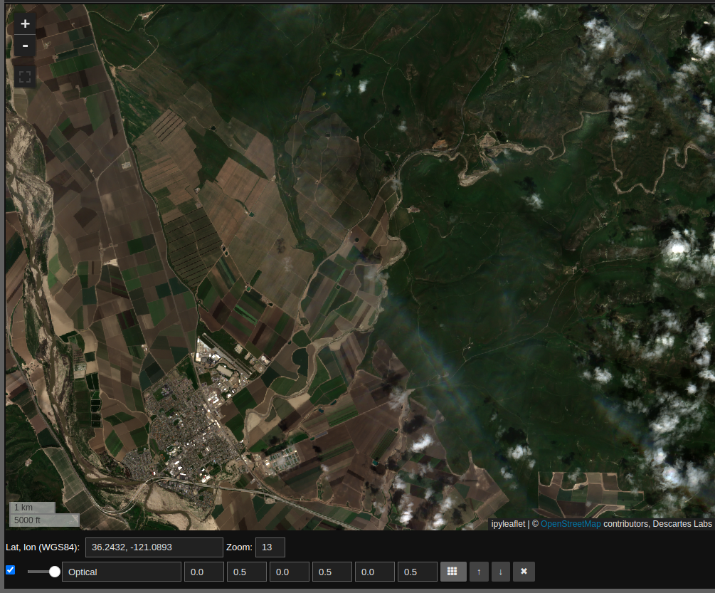
Our first example is to render some optical data on the map. We will start by looking at agriculture in California’s Central Valley. One can pan the map to the area of interest, or programmatically set the map’s location and zoom level with:

m.center = 36.2431, -121.0892
m.zoom = 13

In the above code snippet the first line sets the map’s center to the specified latitude and longitude, while the second line sets the zoom level of the map where the higher the number the more the map is zoomed in. Once we evaluate a notebook cell with the map variable we can view the interactive component, note that we have not yet added any imagery layers to our viewport

Mosaics

Now we will start to work with image data. We instantiate one of the most basic Dynamic Compute objects, a Mosaic, with the following code:

sentinel_2_mosaic = dc.Mosaic.from_product_bands(
  "esa:sentinel-2:l2a:v1",
  "red green blue nir",
  start_datetime="2023-03-01",
  end_datetime="2023-05-01"
)

The above code creates a Mosaic with the following parameters:

"esa:sentinel-2:l2a:v1" is the name of the Descartes Labs Catalog Product we wish to use. This particular product is optical imagery from ESA’s Sentinel-2 program, details about this product can be found here.
"red green blue nir" is a space-separated list of Bands we would like.
start_datetime="2023-03-01" indicates that we should only consider Sentinel-2 imagery collected on or after March 1, 2023.
end_datetime="2023-05-01" indicates that we should only consider Sentinel-2 imagery collected on or before May 1, 2023.

The variable sentinel_2_mosaic is now a Mosaic object representing these selections. Note that the sentinel_2_mosaic variable is not specific to any geographic location, and, by itself, does not contain any geographic data.

A Mosaic object is used to combine data within the specified parameters to create a single layer. Where there are multiple data, the most recent is used.

Accessing Data

To access data we need to provide a geographic area, and there are two ways to do this. First, we can render the data on the map. The map can render three bands, which are assumed to be red, green and blue, or a single band in conjunction with a colormap. We pick the desired bands for viewing from the mosaic with the pick_bands function as follows:

rgb = sentinel_2_mosaic.pick_bands(
  "red green blue"
  )

The variable rgb is another Mosaic and contains only the red, green and blue bands. We can render this on our map with the visualize function as follows:

rgb.visualize(
  "Optical", m, scales=[[0, 0.5], [0, 0.5], [0, 0.5]]
  )

The parameters here are:

“Optical”, which is the name of the layer on the map.
“m”, our dc.map object, which is the map on which to display the data.
scales=[[0, 0.5], [0, 0.5], [0, 0.5]] specifies the scalings for the red green and blue bands. Note that the input data can exceed these bounds, and anything below or above these bounds will be rendered as zero or the maximum, respectively, for the band in question.

With this one should see Sentinel-2 optical imagery on the map as follows:

In response to panning and zooming, the map will request relevant data associated with the rgb Mosaic object. The second way to access data is to request it as an array using the compute function as follows:

result = rgb.compute(m.geocontext())

The compute function takes a single argument, the geocontext. The geocontext contains the coordinate system and the resolution. The dc.map object can generate a geocontext for the current map view via dc.map.geocontext(). Data can be accessed with result.ndarray

result.ndarray.shape
##(3, 400, 939)

Operations

We can perform operations on data in a very natural way. To demonstrate this we begin by accessing single bands within the sentinel_2_mosaic Mosaic:

red = sentinel_2_mosaic.pick_bands("red")
nir = sentinel_2_mosaic.pick_bands("nir")

This creates two new single band mosaics red and nir – nir referring to the near infrared band. We can use these to compute NDVI as follows:

ndvi = (nir - red)/(nir + red)

The math operations +, -, and / can be applied to the red and nir mosaics to generate a new Mosaic called ndvi. As with the rgb mosaic, we can visualize this. Unlike rgb, ndvi has a single band, so visualization requires an additional colormap parameter as follows:

ndvi.visualize("NDVI", m, scales=[[0, 0.8]], colormap='turbo')

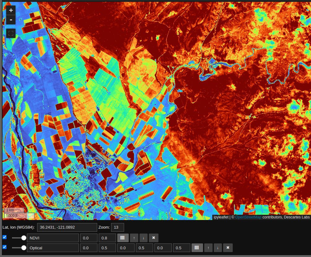
Note that the NDVI layer is computed on the fly in response to changes in the map window. We can also use the NDVI layer to select regions of interest as follows:

vegetation_rgb = rgb.mask(ndvi < 0.3)
vegetation_rgb.visualize("Vegetation", m, scales=[[0, 0.5], [0, 0.5], [0, 0.5]])

By unchecking the “Optical” and “NDVI” layers we see the Sentinel-2 optical imagery for areas where NDVI suggests vegetation.

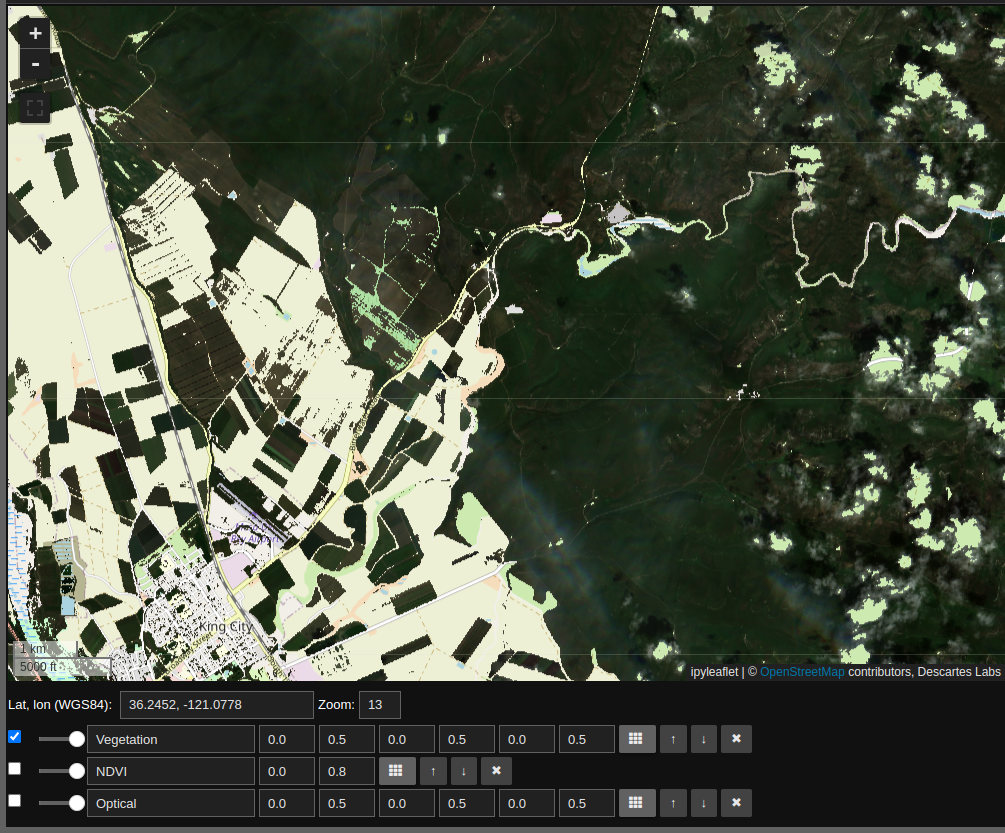
To recap: this layer computes NDVI, uses this quantity to create a mask, and finally renders the RGB layers for the non-masked regions. All of this is done on the fly, and can be applied to any map view.

ImageStack

The Dynamic Compute ImageStack provides a means to access time resolved data. In this example we will create a simple water mask using Sentinel-2 imagery through the same time period.

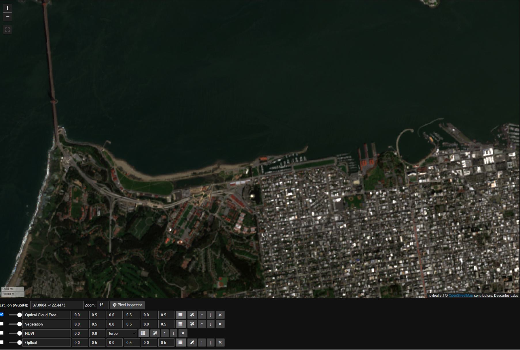
First we’ll set the map view to San Francisco, note the cloud cover in our original Mosaic:

m.center = 37.8084, -122.4473
m.zoom = 15

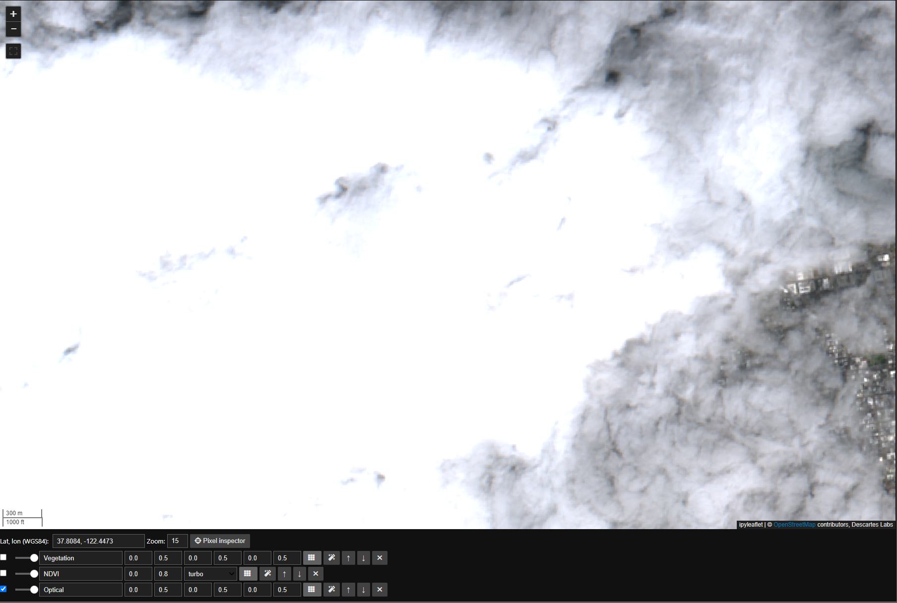
We will address the cloud coverage by first creating an ImageStack in much the same way we created a Mosaic:

sentinel_2_image_stack = dc.ImageStack.from_product_bands(
    "esa:sentinel-2:l2a:v1",
    "red green blue nir",
    start_datetime="2023-03-01",
    end_datetime="2023-05-01"
).filter(lambda x: x.cloud_fraction < 0.1)

Note that we called ImageStack.filter to remove any images that are above a specified cloud_fraction.

Next we will create a composite Image off of this ImageStack. The argument to the function median is axis="images", which indicates that we take the median over the images.:

composite_rgb = sentinel_2_image_stack.pick_bands('red green blue')
composite_rgb.median(axis='images').visualize(
  'Optical Cloud Free', m, scales=[[0, 0.5], [0, 0.5], [0, 0.5]]
  )

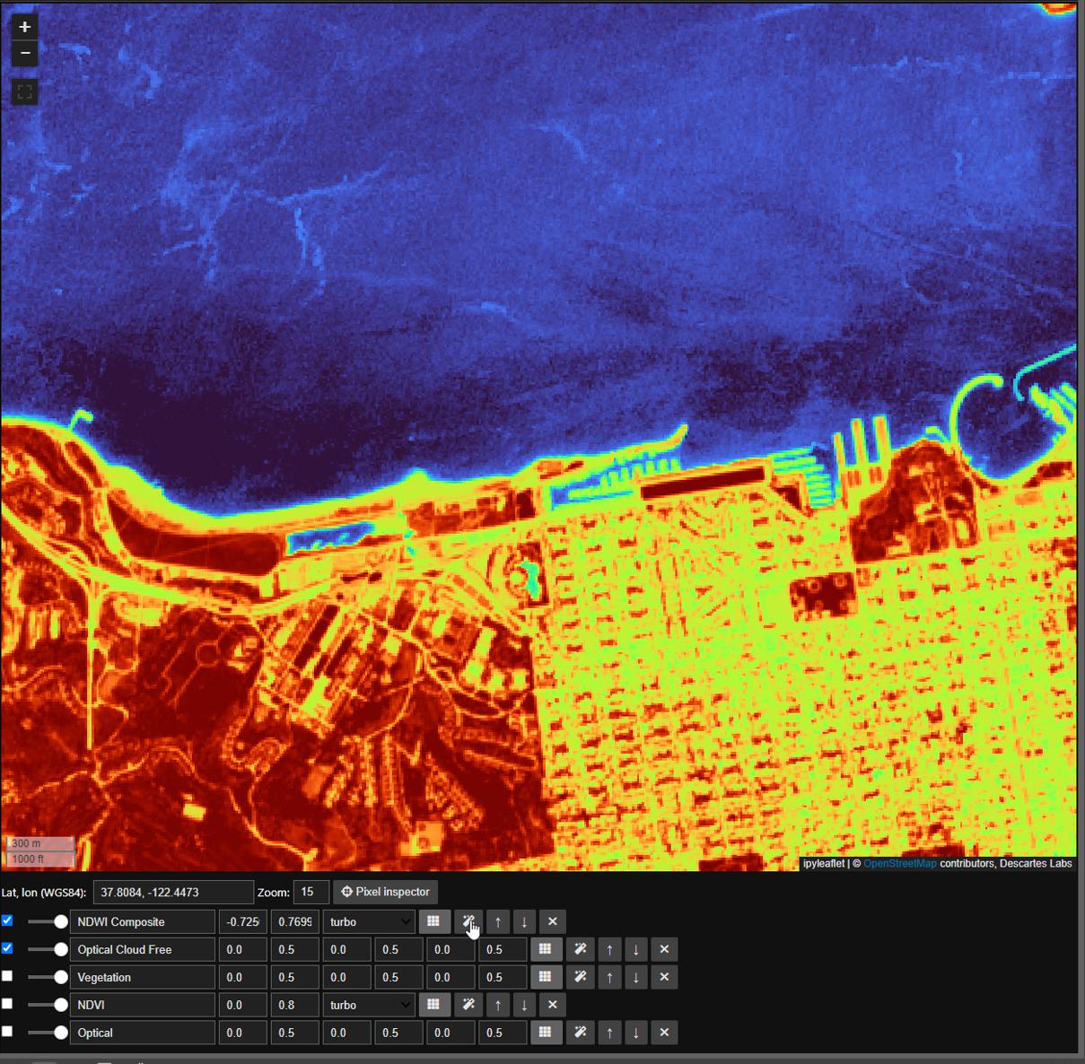
Sentinel-2 in San Francisco without Clouds

Next we will calculate Normalized Difference Water Index, or ndwi, similar to ndvi, using the nir and green bands

composite_nir, composite_green = sentinel_2_image_stack.unpack_bands('nir green')
composite_ndwi = (composite_nir - composite_green) / (composite_nir + composite_green)
composite_ndwi.median(axis='images').visualize('NDWI Composite', dc.map, colormap='turbo')

Here we will take advantage of both the autoscale and pixel inspector tools in Dynamic Compute to visualize and determine a threshold to mask by. The autoscale tool will automatically apply a linear 2% stretch to our dataset and the pixel inspector allows you to select points through which you want to sample imagery values.

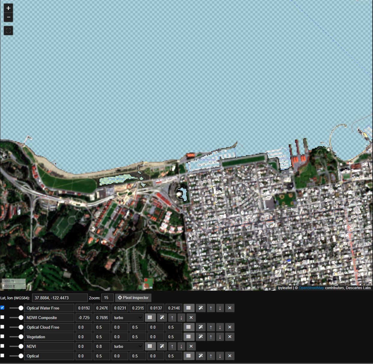
Now that we have settled on a threshold, in this case we’ll use a round 0, we can finally mask our ImageStack just like any Mosaic. Here we will mask to min ndwi, note that all masked portions are now represented by a checkerboard

water = composite_ndwi.min(axis='images') < 0
composite_rgb.mask(water).pick_bands('red green blue').median(axis='images').visualize('Optical Water Free', m)