Vector ⥂

Vector is a catalog for vector data. It enables users to store, query, and display vector data — which includes everything from fault lines to thermal anomalies to material spectra to ML detections.

This quick-start guide provides examples to demonstrate some of the basic features of Vector. This guide’s prerequisite is a notebook environment that includes the Descartes Labs Python client and supports ipyleaflet. Vector tables consist of features, which themselves consist of a geometry and properties. The following geometry types are supported: Point, MultiPoint, LineString, MultiLineString, Polygon, MultiPolygon.

Installation

If you are using Workbench, Vector will come already installed on your Python environment. If you are using another environment, install the Descartes Labs client from PyPI by running

$ pip install descarteslabs

If you wish to use the visualization features, then be sure to install ipyleaflet also, or use the viz extra.

Getting Started

Vector is available within the Descartes Labs client and can be imported into a notebook with the following:

import descarteslabs as dl
from descarteslabs.utils import Properties
from descarteslabs.vector import Table, models
from pydantic import Field
from typing import Union, Optional

Creating a Vector Table

Vector tables to which a user has read access at minimum can be listed by using the list() method.

for table in Table.list():
  print(table.id)

In the above code example, the id property is being accessed with each iteration, which will return the Vector table ID. Vector table IDs must be unique within a given organization.

As this is an example notebook and table IDs must be unique, any existing Vector table with the same table ID for this example will first be deleted.

orgname = dl.auth.Auth().payload["org"]
for table in vector.Table.list():
    if table.id == f"{orgname}:us-counties":
        print(f"Deleting {table}")
        table.delete()

In the code above, Vector tables are listed and iterated over. If a table already exists with the table ID equivalent to us-counties, it will be deleted by calling the delete() method.

With any potential duplicate Vector tables now deleted, a Vector table can created. Vector allows the user to define a custom schema/model for each Vector table. Below is the list of predefined base models which should be inherited to define the schema. If your data does not contain a geometry column (i.e. aspatial), the model should inherit from VectorBaseModel which will inherit the required UUID column. If your data does contain a geometry column, the appropriate model for the given geometry type must be selected, which will inherit both the required UUID and geometry columnns. If a multi-geometry model is selected, all geometries will be promoted to multi-part.

models.VectorBaseModel # aspatial/tabular data only
models.PointBaseModel # data containing point geometries
models.MultiPointBaseModel # data containing multi-point geometries
models.PolygonBaseModel # data containing polygon geometries
models.MultiPolygonBaseModel # data containing multi-polygon geometries
models.LineBaseModel # data containing line geometries
models.MultiLineBaseModel # data containing multi-line geometries

Once the appropriate base model has been determined, a custom model/schema can be created by inheriting the base model. Column names and data types can then be attributed to the custom model/schema. Below is the complete list of accepted data types.

class CustomModel(models.VectorBaseModel):
    column_a: str
    column_b: int
    column_c: float
    column_d: datetime.date
    column_e: datetime.datetime
    column_f: list
    column_g: dict
    column_h: bool
    column_i: List
    column_j: List[str]
    column_k: List[int]
    column_l: List[float]
    column_m: List[bool]
    column_n: List[dict]

By default, columns are not nullable. However, you can define a column to be nullable by wrapping the data type with typing.Optional[data_type] or typing.Union[data_type, None]. If the Vector table has a geometry column, a spatial index will be created automatically. To specify the creation of an index on another column, use pydantic.Field. Examples for both cases are provided below.

class CustomModel(models.VectorBaseModel):
    column_a: Optiona[str] = Field(json_schema_extra={"index": True})
    column_b: Union[int, None]

For a more realistic example, we will create a Vector table pertaining to US counties. The custom model/schema, CountyModel, inherits from MultiPolygonBaseModel. Since the UUID and geometry columns are inherited from the base model, we only need to define the additional columns. Invoking the create() method will create the actual table. This method requires a product ID, which will be prefixed with YOURORGNAME:, a table name, and a table model/schema. Upon successful creation, a Table object will be returned.

CountyModel(models.MultiPolygonBaseModel):
  STATEFP: str = Field(json_schema_extra={"index": True})
  COUNTYFP: str
  COUNTYNS: str
  AFFGEOID: str
  GEOID: str
  NAME: str
  LSAD: str
  ALAND: int
  AWATER: int

table = Table.create(
  product_id="us-counties", # ID for the table
  name="US Counties",  # Name for the table
  owners=[f"org:{orgname}"], # Table owners
  model=CountyModel
)

Ingesting Data

With the Vector table created, the table can be populated with features using the following code:

import requests
url = "https://gist.githubusercontent.com/sdwfrost/d1c73f91dd9d175998ed166eb216994a/raw/e89c35f308cee7e2e5a784e1d3afc5d449e9e4bb/counties.geojson"
response = requests.get(url)
feature_collection = response.json()
gdf = gpd.GeoDataFrame.from_features(feature_collection["features"], crs="EPSG:4326")
gdf = table.add(feature_collection)

In the above code snippet, a GeoJSON feature collection was downloaded from a webpage. The feature collection was then converted to a GeoDataFrame and ingested to the table with the add() method. Adding features will return a GeoPandas.GeoDataFrame with UUID attribution. If the Vector table were aspatial (i.e. no geometry column), a Pandas.DataFrame with UUID attribution would returned.

Querying Data

TableOptions

Vector products can be filtered/queried by specifying a property_filter, columns, and aoi. In the case of Vector, property_filter, columns, and aoi are collectively referred to as TableOptions. Subsequent method calls on the Table object will honor these options.

property_filter: Property or column filter for the query. Default is no filter.
columns: A subset of columns to return with each query. Default is all columns will be returned.
aoi: Spatial filter for the query. Default is no spatial filter.

Setting the TableOptions can be done during initialization of a Table object:

# initialize properties
p = Properties()

table = Table.get(
  f"{orgname}:us-counties",
  property_filter=p.NAME == "Santa Fe",
  columns=["geometry", "STATEFP", "NAME"],
)

df = table.collect()

updated after initialization:

table = Table.get(f"{orgname}:us-counties")
table.options.property_filter=p.NAME == "Santa Fe"
table.options.columns=["geometry", "STATEFP", "NAME"]

df = table.collect()

or overwritten entirely:

options = TableOptions(
  f"{orgname}:us-counties",
  property_filter=p.NAME == "Santa Fe",
  columns=["geometry", "STATEFP", "NAME"],
)
df = table.collect(override_options=options)

The table options can be reset to default at any point using the reset_options() method.

table.reset_options()

Querying

As seen from the previous examples, calling the collect() method will execute a query based on the specified TableOptions. Upon successful completion, a GeoPandas.GeoDataFrame or Pandas.DataFrame will be returned. If the table was spatial (i.e. has a geometry column) and the columns option was not set or the geometry column was included in the columns option, a GeoPandas.GeoDataFrame will be returned; otherwise, a Pandas.DataFrame will be returned. The DataFrame will only contain data for the columns specified in the options. More complex queries can be constructed as seen below:

aoi = {
    "type": "Polygon",
    "coordinates": [
        [
            [-109.63936670604541,33.07321249994284],
            [-99.18198027219883,33.07321249994284],
            [-99.18198027219883,39.037426282400816],
            [-109.63936670604541,39.037426282400816],
            [-109.63936670604541,33.07321249994284]
        ]
    ],
}

table = Table.get(
  f"{orgname}:us-counties",
  aoi=aoi,
)

df = table.collect()
df

In the example above, invoking the collect() method returns a GeoPandas.GeoDataFrame containing rows (counties) that intersected our AOI. Since we did not set the columns option, all columns will be returned.

table.reset_options()
table.options.property_filter = p.NAME == "Santa Fe"
gdf = table.collect()
gdf

In the example above, we have reset the TableOptions which has cleared the AOI we previoulsy specified. Now we have set the property filter to only include rows (counties) named Santa Fe.

table.reset_options()
table.options.property_filter = p.STATEFP == "49"
table.options.aoi = aoi
gdf = table.collect()
gdf

US Counties that Intersect AOI and have FIPS Code Equal to 49

Lastly, any combination of table options can be constructed to define a query. In above example, we have reset the table options which has cleared the previous property filter. We then set a new property filter and AOI to only include rows (counties) that are in Utah (FIPS 49) and intersect our AOI.

Visualization

Working within a Python notebook, Vector tables can be visualized by calling the visualize() method which will add a VectorTileLayer to the provided map display. Note this method is only applicable to spatial Vector tables.

m = ipyleaflet.Map(
    scroll_wheel_zoom=True,
    center=(44.5, -103)
)
m.zoom = 3
m

table = Table.get(f"{orgname}:us-counties")

table.visualize("US Counties", m)

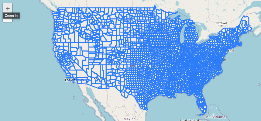
In this example, an ipyleaflet map has been created centered over the US. Invoking the visualize() method will add a layer displaying the features of the table to the map.

Filtering Tiles

Similar to the query examples above, Vector visualization also supports the use of TableOptions; however, only the property filter and columns will be honored.

p = Properties()

table.options.property_filter = p.STATEFP == 35

# add layer style
vector_tile_layer_styles = {
    "default": {
        "fill": "true",
        "fillColor": "#00ff00",
        "color": "#000000",
        "fillOpacity": 0.5,
    }
}

table.visualize(
    name="New Mexico Counties",
    map=m,
    vector_tile_layer_styles=vector_tile_layer_styles
)

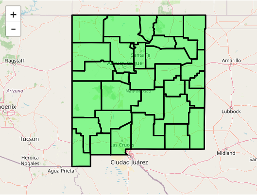
In this example, the visualize() method has been invoked with a property filter and layer style. Instead of visualizing all US counties, only counties with a state FIPS code of 35, e.g. New Mexico. The layer added to the map display will be formatted according to the vector_tile_layer_style.

Deleting Tables

To delete a table, simply invoke the delete() method on a table object.

try:
    table = Table.get(f"{orgname}:us-counties")
    table.delete()
except:
    print("Table does not exist!")

In this example, retrieving and deleting a table are encapsulated in a try/except block. When retrieving a table, if the table does not exist, an error is raised.